Understanding Self-Attention from First Principles

Ever since the dawn of NLP, there has been a constant pursuit of finding a way to convert human-readable text into machine-understandable numbers.
Some of the earliest strides in this direction were techniques such as One-Hot Encoding, Bag of Words (BoW), and TF-IDF. These methods were undoubtedly important milestones and laid the foundation for many advances that followed. However, each of them came with its own set of limitations. These limitations kept researchers in the field curious and motivated to develop something better than the existing solutions.
The next major milestone was the introduction of embeddings.
Classical embedding methods such as Word2Vec, GloVe, and FastText represented words using dense vector representations that captured meaningful semantic relationships. Unlike sparse representations such as one-hot encoding or Bag of Words, embeddings placed semantically related words closer together in vector space. They do a remarkably good job of preserving the essence of a word, phrase, or even an entire sentence within a fixed-dimensional vector space.
However, these embeddings had an important limitation: they were static.
Once trained, a word was assigned a single vector representation that remained unchanged regardless of the context in which the word appeared.
Because of this static nature, embeddings could inherit biases present in the training data.
Consider an embedding model trained on a dataset containing 10,000 sentences about the word Apple. Suppose 8,000 of those sentences refer to the fruit, while only 2,000 refer to the technology company.
As expected, the learned representation of the word Apple would be pulled heavily toward the fruit sense, because that is the meaning it encountered far more often during training. The technology company sense would still leave some trace in the vector, but the two meanings would be compressed into a single compromise representation, one that does not cleanly capture either usage.
The fundamental problem is not simply that one meaning dominates. The deeper problem is that both meanings are collapsed into one vector. That single vector must serve as the representation of Apple in every sentence, regardless of whether the surrounding context is talking about a fruit basket or a smartphone launch event.
And since these embeddings are static, there is very little they can do to adapt themselves to the context of a particular sentence. Once trained, the same vector representation is reused again and again. The world needed a solution to this problem.
What was needed was a mechanism capable of producing contextualized representations. In other words, the representation of a word should not remain fixed. Instead, it should be able to adapt itself based on the context in which that word is being used.
Ideally, the same word should be allowed to have different vector representations when it carries different meanings.
For example, consider the following two sentences:
- Apple is a red-colored fruit.
- Apple makes good phones.
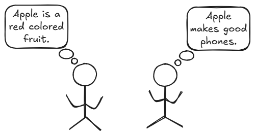
Although the word Apple appears in both sentences, it clearly refers to two entirely different things. Therefore, the embedding generated for Apple in the first sentence should be different from the embedding generated for Apple in the second sentence.
In other words, the representation of a word should be influenced not only by the word itself but also by the words surrounding it. This is exactly what contextualized representations aim to achieve.
One of the key mechanisms that made this possible is self-attention.
Self-attention can be regarded as the core building block of the Transformer architecture, which in turn powers nearly all modern large language models and many of the NLP systems we use today.
And it is also the topic of this very blog.
But what exactly is self-attention?
At a high level, self-attention is a mechanism that takes static embeddings as input and produces contextualized representations as output.
For now, you can think of self-attention as a function. We provide it with a sequence of static embeddings, and it performs a series of computations internally. Once those computations are complete, it outputs a new sequence of embeddings, where each embedding has been enriched with contextual information gathered from the other words in the input sequence.
In other words, self-attention transforms static embeddings into contextualized representations.
This is precisely what allows the same word to receive different representations depending on the context in which it appears.
A Running Example
Let us now dissect this self-attention function and take a closer look at what this mechanism really is at its core.
To build a better understanding and maintain a smoother flow throughout this blog, we will work with a running example and carry it forward as we gradually uncover the different components of self-attention.
Consider the following two phrases:
- Money bank grows
- River bank flows
These phrases may not sound particularly natural in everyday language, but they are more than sufficient for building an intuition for how self-attention works.
As you might notice, both phrases contain a common word: bank.
However, the word bank is being used in two entirely different contexts.
In the first phrase, Money bank grows, the word bank refers to a financial institution where money is stored.
In the second phrase, River bank flows, the word bank refers to the land alongside a river.
Now, had we gone down the traditional static-embedding route, the vector representation of the word bank would have been exactly the same in both phrases, despite the fact that the meanings are completely different.
For example, suppose our embedding model represents bank using the following four-dimensional vector:
Then both occurrences of bank would receive this exact same representation.
Clearly, this is not an ideal situation. Even though the word is the same, its meaning changes depending on the surrounding context. Ideally, the representation of bank in the first phrase should be different from the representation of bank in the second phrase.
And this is precisely the problem that self-attention is designed to solve.
Manually Weighting the Context
So, we abandon the idea of relying solely on static embeddings and instead adopt a new approach.
Let us zoom in on the word bank in both phrases.
In the phrase Money bank grows, the contextual embedding of the word bank does not come exclusively from the word bank itself. Instead, it can be thought of as being influenced partly by the word money, partly by the word bank, and partly by the word grows.
In other words, the final representation of bank is constructed by gathering information from all the words present in the input sequence.
To make this idea concrete, let us assign some hypothetical weights to these contributions. These weights represent how much each word contributes to the contextual meaning of bank. Furthermore, all of these weights must add up to 1.
For the phrase Money bank grows, let us assume:
- money contributes 0.2
- bank contributes 0.7
- grows contributes 0.1
Notice that:
Similarly, consider the phrase River bank flows.
Once again, the contextual embedding of bank is not derived solely from the word bank. Instead, it is influenced by all the words in the phrase.
Let us assume the following contributions:
- river contributes 0.5
- bank contributes 0.4
- flows contributes 0.1
And once again:
Notice something interesting here.
Although the word bank appears in both phrases, the contributions coming from the surrounding words are different. In the first phrase, money exerts a stronger influence, whereas in the second phrase, river exerts a stronger influence.
As a result, the final contextual embedding of bank will be different in the two phrases, allowing the model to distinguish between the financial institution and the riverside landform.
Of course, this process is not limited to the word bank.
In a self-attention layer, every word computes how much it should depend on every other word in the sequence, including itself.
So, just as we calculated how much the word bank depends on money, bank, and grows, we can perform the same calculation for every other word as well.
For the phrase Money bank grows, let us assume the following dependencies:
| Word | Money | Bank | Grows |
|---|---|---|---|
| Money | 0.6 | 0.3 | 0.1 |
| Bank | 0.2 | 0.7 | 0.1 |
| Grows | 0.2 | 0.5 | 0.3 |
For example, the first row tells us that the contextual embedding of money is formed using:
- 60% information from money itself,
- 30% information from bank,
- 10% information from grows.
Similarly, for the phrase River bank flows, let us assume:
| Word | River | Bank | Flows |
|---|---|---|---|
| River | 0.7 | 0.2 | 0.1 |
| Bank | 0.5 | 0.4 | 0.1 |
| Flows | 0.3 | 0.1 | 0.6 |
Again, every row sums to 1.
These values tell us how much information each word gathers from the other words in the sequence while constructing its contextual embedding.
Notice that we are no longer asking:
"What is the embedding of this word?"
Instead, we are asking:
"How much information should this word collect from every other word before constructing its final contextual embedding?"
And that question lies at the heart of the self-attention mechanism.
From Words to Embeddings
So far, we have been talking about words influencing other words. For example, we said that the word money depends partly on money, partly on bank, and partly on grows.
While this intuition is useful, words themselves are not what neural networks operate on.
A much better way of representing words in NLP is through embeddings.
Therefore, instead of saying that the contextual embedding of money is formed using contributions from the words money, bank, and grows, we can say that it is formed using contributions from the embeddings of those words.
In other words, the contextual embedding of money can be viewed as a weighted combination of:
- the embedding of money,
- the embedding of bank,
- and the embedding of grows.
The weights remain exactly the same as before; the only difference is that we are now applying them to embeddings rather than to the words themselves.
For example, using the dependency values we assumed earlier, the contextual embedding of money can be expressed as:
where , , and denote the embedding vectors of the corresponding words.
Similarly, the contextual embedding of bank would be formed by taking a weighted combination of the embeddings of money, bank, and grows using the attention weights assigned to bank.
The exact same process is repeated for every word in both sentences.
This is a very important shift in perspective.
Self-attention does not directly combine words. Instead, it combines the vector representations of those words, producing a new set of embeddings that now contain contextual information from the surrounding words.
Establishing Notation
Before progressing any further, let us establish some notation that we will use throughout the rest of this blog.
Let
denote the original embedding of a word.
Similarly, let
denote the new contextual embedding produced by the self-attention mechanism.
Our goal throughout the remainder of this blog is to answer a single question: how are these new embeddings calculated?
To build some intuition, let us revisit the phrase Money bank grows.
Using the contribution weights that we assumed earlier, the contextual embedding of the word money can be written as:
Similarly, the contextual embedding of the word bank can be written as:
And the contextual embedding of the word grows becomes:
Notice what is happening here.
Each new embedding is formed by taking a weighted sum of the embeddings of all the words present in the sentence. Some words contribute more, while others contribute less, but every word is allowed to influence every other word.
A quick note about the coefficients such as , , and .
These values represent how much information a word chooses to gather from another word while constructing its contextual embedding. Larger values indicate a stronger influence, whereas smaller values indicate a weaker influence.
For example,
tells us that the new representation of money is influenced most heavily by its own original embedding, while also incorporating some information from bank and grows.
Throughout this blog, all embeddings will be assumed to be -dimensional vectors.
The central idea to remember is that the new embedding of a word is obtained by taking a weighted combination of the embeddings of all the words in the sentence.
There is a small but important consequence of this worth noting before moving on. The coefficients , , and are not fixed properties of the word money. They depend on whichever words happen to be sitting alongside it. Change the surrounding words, and these weights change with them; change the weights, and the weighted combination they produce changes too. This is precisely why the same word can end up with a different contextual embedding from one sentence to the next: it is not the word that changes, but the company it keeps.
Where Do the Weights Come From?
At this point, a natural question arises.
We have been assuming the existence of weights such as , , and , but where do these values actually come from?
We still need a way to determine how much information one word should gather from another.
Intuitively, if two words are highly related in a particular context, we would like them to influence one another more strongly. Conversely, if two words are largely unrelated, their influence should be weaker.
One of the simplest and most effective ways of measuring this relationship between two vectors is the dot product.
In general, if two vectors point in similar directions in the vector space, their dot product tends to be large. Conversely, if they are dissimilar, their dot product tends to be smaller.
For now, it is useful to think of the dot product as a measure of similarity, since the embeddings we are working with at this stage are still static and untrained. Once we introduce learnable Query and Key projections later in this blog, this interpretation will need to be loosened. After training, a high dot product is better understood as a learned relevance score rather than literal semantic similarity. Two tokens can end up with a high attention score even if their original embeddings are not semantically similar at all; what matters is that the model has learned that paying attention to that interaction is useful for the task at hand.
Building on this intuition, let us attempt to compute the contextual embedding of the word bank using dot products directly.
A first attempt might look something like this:
Let us interpret what this equation is doing.
The term
measures the similarity between the embeddings of money and bank.
Similarly,
measures how similar bank is to itself, and
measures the similarity between grows and bank.
These similarity scores are then used to determine how much influence each embedding should have when constructing the new contextual embedding of bank.
Conceptually, this is very close to what we want: words that are more relevant to bank should contribute more to its final representation, while less relevant words should contribute less.
Let us write this a little more cleanly:
Assume that the dot products inside the square brackets evaluate to the scalars , , and respectively.
Our equation now becomes:
Notice that , , and are scalar values. This is expected because the dot product of two vectors produces a scalar.
However, there is still a problem.
These values are not normalized. They can take on arbitrary magnitudes and are not guaranteed to sum to 1. As a result, they cannot yet be interpreted as meaningful contribution weights.
We therefore need a way to normalize them.
A very effective way of doing this is by passing these values through a Softmax function.
More specifically, we apply Softmax to the set of scores:
The Softmax function transforms these raw scores into normalized weights:
where
These -values can now be interpreted as contribution weights, indicating how much information the word bank should gather from each word in the sentence while constructing its contextual embedding. We use the symbol here, rather than , to keep these attention weights clearly distinct from the projection matrices , , and that we will introduce shortly.
Replacing the unnormalized scores with their normalized counterparts, we obtain:
This should look very familiar.
Earlier in the blog, we manually assumed values such as , , and . We now have a mechanism for computing those values automatically. The dot products generate similarity scores, and the Softmax function converts those scores into normalized weights that can be used to construct the new contextual embedding.
Putting It All Together
Now let us move forward.
According to our formula, the next step is straightforward.
We multiply the normalized weights , , and with their corresponding embeddings:
Since each -value is a scalar and each embedding is an -dimensional vector, the result of each multiplication is again an -dimensional vector.
Once these weighted embeddings have been computed, we simply add them together:
The resulting vector is the new contextual embedding of the word bank in the phrase Money bank grows.
Notice what has happened.
The original embedding of bank has now been enriched with information gathered from the other words in the phrase. Instead of depending solely on its own static embedding, it now incorporates contextual information from money and grows as well.
This newly generated embedding is therefore context-aware and dynamic.
Of course, we do not perform this process only for the word bank.
The exact same procedure is repeated for every word in the input sequence. In our running example, we would similarly compute new contextual embeddings for money and grows. Likewise, for the second phrase, we would compute contextual embeddings for river, bank, and flows.
By the end of this process, every word in the sequence receives a new embedding that has been influenced by the words surrounding it.
And that is precisely the output produced by the self-attention mechanism.
The following diagram illustrates exactly this: each word generating its own similarity scores against every other word, passing those scores through Softmax, and then combining the embeddings accordingly to produce , , and :
A quick note on notation before moving on: is simply a shorthand for . The two are the same object. is just a more compact way of writing the contextualized embedding once diagrams and matrix notation enter the picture, and the two notations will be used interchangeably from here on.
Two Important Observations
I hope you are following along so far.
Using our running example, we have gradually arrived at a mechanism that looks remarkably similar to what would eventually become self-attention.
Before moving any further, let us pause for a moment and look closely at what we have just built.
There are two important observations to make about this mechanism.
Observation 1: Everything can be computed in parallel
If you look carefully at the mechanism we have constructed so far, every computation is independent of the others.
The similarity score between one pair of embeddings can be computed without waiting for the similarity score of any other pair. Likewise, the attention weights for one word can be computed independently of the attention weights for every other word. And once those weights have been obtained, the contextual embedding of a word can be formed without needing the contextual embeddings of the remaining words.
As a result, there is no inherent sequential dependency in the computation.
Unlike recurrent architectures, which process tokens one after another, the mechanism we have built allows every word in the sequence to perform its computations simultaneously.
This means that instead of processing:
Money → bank → grows
one word at a time, we can process the entire sequence in parallel.
This property turns out to be extremely important.
Modern hardware such as GPUs is highly optimized for performing large numbers of mathematical operations simultaneously. Since the computations in our attention mechanism do not depend on one another, they can be expressed as matrix operations and executed very efficiently in parallel.
This parallelism is one of the key reasons attention-based architectures scale so effectively to large datasets and long sequences.
However, this advantage comes with an important trade-off.
Because every word is processed simultaneously, the mechanism itself has no built-in notion of sequence order.
From its perspective, the phrases
Money bank grows
and
Grows bank money
contain exactly the same set of embeddings.
The mechanism can determine how strongly words should influence one another, but nothing in the computations we have described so far tells it which word appeared first, second, or third.
In other words, the attention mechanism by itself does not encode positional information.
Fortunately, Transformer architectures solve this problem through a technique known as positional encoding, which injects information about token positions into the embeddings before attention is applied.
We will not cover positional encoding in this blog, but it is worth keeping in mind that attention alone is not sufficient for modeling word order.
Scaling to Longer Sequences
Up until now, we have intentionally described everything from the perspective of individual words.
For example, when constructing the contextual embedding of bank, we manually computed similarity scores, converted those scores into attention weights, and then used those weights to form a weighted combination of embeddings.
This word-by-word view is extremely useful because it exposes the underlying intuition.
However, Observation 1 reveals something important.
None of the computations we performed actually need to be carried out one word at a time.
The similarity scores for all pairs of words can be computed simultaneously.
The attention weights for all words can be computed simultaneously.
And the contextual embeddings for all words can be constructed simultaneously.
In practice, we therefore replace the word-by-word view with a matrix-based formulation that performs exactly the same computations for the entire sequence at once.
Matrices are not introducing a new mechanism.
They are simply a compact way of expressing the same operations we have already derived.
Recall our running example:
Money bank grows
We can stack the embeddings of all three words into a single embedding matrix:
This is a matrix, where:
- is the number of words in the sequence.
- is the dimensionality of each embedding vector.
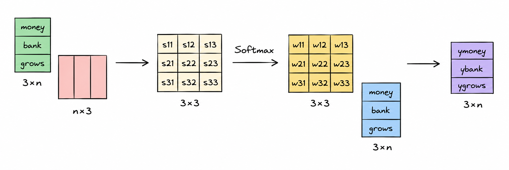
The diagram below expresses the same attention mechanism we previously built, but now in matrix form.
Observation 2: There are no learnable parameters
There is another interesting property of the mechanism we just constructed.
Notice that nowhere in our formulation did we introduce any trainable weights or learnable parameters. To be precise about what this claim does and does not cover: it is the attention computation itself (the dot products and the Softmax) that introduces no new trainable weights. The embeddings that we feed into this mechanism may very well have been learned elsewhere, for instance by a Word2Vec-style training process. The attention mechanism does not add anything on top of that; it simply operates on whatever embeddings it is given.
Because the attention computation contains no learnable parameters, it cannot adapt its behavior to a specific downstream task. It can contextualize tokens, allowing each word to gather information from the words around it, but the representations it produces are not shaped by any task-specific objective.
This matters because many real-world tasks require more than contextualization. A parameter-free attention mechanism can redistribute information that is already present in the embeddings, but it cannot learn which relationships matter for a particular task. Whether two tokens should influence each other strongly is something that needs to be learned from data. Without trainable weights, the model has no way to discover that subject-verb agreement matters for grammar, that sentiment-bearing words should dominate a sentiment-analysis decision, or that a question word should attend strongly to the span containing its answer. These are precisely the kinds of task-specific patterns that translation, summarization, sentiment analysis, and question answering depend on.
In other words, gathering information from surrounding words is a necessary first step, but without learning from data, the model has no way of knowing which of those words actually matter for the task at hand.
The Same Embedding, Three Different Roles
Upon observing this architecture more carefully, we arrive at an important realization.
The mechanism we have built so far is capable of generating contextualized representations. However, these representations are still fairly general-purpose. They are not optimized for any particular task because the architecture contains no learnable parameters.
If we want the model's contextualized representations to be shaped by what it learns from data, then the model must be able to learn from data.
And for a model to learn from data, it needs learnable parameters.
In other words, we need to introduce weights and biases into the architecture.
Before we do that, however, let us make an interesting observation.
Notice that the same embedding of a word is being used three different times while computing its contextual embedding.
Consider the leftmost block, where we are trying to generate the contextual embedding of the word money, namely .
If you look closely, the embedding appears three times:
- Once in the green box,
- Once in the pink box,
- And once in the blue box.
The exact same thing happens for bank and grows.
When generating , the embedding appears in the green box, the pink box, and the blue box.
Likewise, when generating , the embedding appears in all three locations.
This raises an interesting question.
Why are we using the same embedding three times?
The answer is that, although all three boxes contain the same embedding, they are actually playing three completely different roles.
Looking at the leftmost block, where we are trying to generate .
The green embedding is responsible for comparing itself against all other embeddings in the sentence in order to determine how relevant each of them is.
It acts as the querying vector, the representation that drives the similarity computation.
This naturally motivates the name:
Query (Q)
Now let us look at the pink embeddings.
The similarity score between a Query and every other token is computed by comparing the Query against the pink representations. In other words, the pink embedding is the representation against which a Query is matched. A large dot product between a Query and a pink Key indicates high relevance; a small dot product indicates low relevance.
What matters is not that a Key "has meaning" on its own, but rather that the interaction between a Query and a Key produces a meaningful relevance score.
This naturally motivates the name:
Key (K)
Finally, consider the blue embeddings.
Once all the similarity scores have been computed and normalized through Softmax, we obtain the attention weights.
These weights are then used to compute a weighted sum.
And what exactly are we taking the weighted sum of? The blue embeddings.
The blue embeddings are therefore the actual pieces of information that get aggregated together to form the final contextualized representation.
This motivates the final name:
Value (V)
So although we started with a single embedding for every word, we can think of that embedding as simultaneously playing three different conceptual roles:
- Querying other tokens for relevance,
- Being queried against to determine relevance,
- And providing information to be aggregated.
These three roles are what eventually become the Query, Key, and Value vectors used in the Transformer architecture.
Query (Q): The vector that drives the similarity computation: "How relevant is each other token to me?"
Key (K): The vector that is compared against a Query to produce a relevance score. Relevance is determined by the Query-Key interaction, not by the Key alone.
Value (V): The vector containing the actual information that will be aggregated using the attention weights: "What information should I contribute to the final contextualized representation?"
Why Is It Called Self-Attention?
At this point, it is worth pausing to address a question that often arises when people first encounter this mechanism.
Why is it called self-attention?
The answer lies in where the Queries, Keys, and Values come from.
In the mechanism we have been building, all three of these quantities are derived from the same input sequence. When we compute the contextual representation of a word in the phrase Money bank grows, both the query and the things being queried are tokens from that same phrase. Each token attends to all other tokens within the same sequence, including itself.
This is what the word self refers to. The sequence is attending to itself.
This distinguishes self-attention from cross-attention, which is used in the encoder-decoder attention layers of the original Transformer. In cross-attention, the Queries come from one sequence (for example, the sequence being generated), while the Keys and Values come from a different sequence, such as the encoded source sentence. In self-attention, all three come from the same sequence.
Keeping this distinction in mind will make the architecture of the full Transformer considerably easier to understand when you encounter it.
It is worth pausing here to make the division of labor explicit, since it is easy to wonder why we need two separate roles, Key and Value, instead of just one.
The Query asks a question: what is relevant to me? The Key answers on behalf of its token: here is how to judge whether I am relevant to you. Together, the Query and the Key determine where to look. They decide how much attention one token should pay to another. The Value, by contrast, determines what is actually retrieved once that decision has been made. You can think of the Key as an address and the Value as the content stored at that address: the Query-Key interaction is what lets a token find the right addresses to look up, but it is the Value that gets delivered once the lookup is done. Scoring relevance and supplying information are different jobs, so it makes sense that they are handled by different vectors.
The reason a Query-Key dot product is useful is not that it captures semantic similarity in any fixed sense, but that training shapes the Query and Key projection spaces so that a large dot product comes to signal learned relevance. The model is free to map two tokens into Query and Key spaces where they end up well-aligned precisely because attending to one another helps it solve the task, regardless of how similar their original embeddings looked.
If a Query vector and a Key vector produce a large dot product, the model interprets the corresponding token as being important to the querying token. Tokens receiving higher similarity scores will therefore contribute more strongly to the final contextualized representation.
It is also worth appreciating what happens during training. As the model learns, it adjusts the projection matrices and so that tokens which should exchange information tend to develop larger Query-Key similarity scores, while tokens that are less relevant to one another tend to develop smaller scores. In other words, the dot product does not start out as a meaningful relevance signal. It becomes one as the model learns which Query-Key interactions are useful for the task at hand. This is precisely why the dot product is such a powerful mechanism at the core of attention.
So far, we are in a good position.
We have identified the three components that we would like to turn into learnable parameters: Query, Key, and Value.
However, there is still a problem.
Although we have conceptually separated the roles of Query, Key, and Value, they are all still being played by the exact same embedding vector.
For example, when computing the contextual embedding of the word bank, the embedding simultaneously acts as:
- the Query vector,
- the Key vector,
- and the Value vector.
This is not an ideal design.
What we want is a clear separation of concerns.
The information that helps a word ask questions does not necessarily have to be the same information that helps it answer those questions. Similarly, the information that should be aggregated into the final contextual embedding does not necessarily have to be the same information used for similarity matching.
In other words, we would like to have three separate representations:
- one dedicated to querying,
- one dedicated to matching queries,
- and one dedicated to carrying information.
At the same time, we do not want to completely discard the original embedding. After all, the original embedding already contains useful semantic information.
So the natural question becomes: how can we derive three different vectors from a single embedding?
If querying, matching, and carrying information are fundamentally different tasks, it seems unreasonable to force a single vector to perform all three roles simultaneously. What we need is a way to take that one embedding and stretch it into three specialized versions of itself, each tailored to the role it is meant to play.
Before we proceed, it is worth flagging something important.
Up until this point, we have been constructing the contextual representation of a word by taking a weighted sum of the original embeddings of the other words in the sequence. This was a deliberate simplification. The goal was to build a clear intuition for how attention weights are computed and applied, without introducing unnecessary complexity too early.
Once we introduce Query, Key, and Value vectors, the final step changes slightly. Instead of taking a weighted sum of the original embeddings, we take a weighted sum of the Value vectors. You can think of the earlier formulation as a special case of this, one where the Value vectors simply are the original embeddings. The more general version, where Values are produced by a separate learned projection, gives the model considerably more flexibility.
It is worth being explicit about what is and is not changing here. The attention mechanism itself stays exactly the same: we still compute relevance scores between tokens, we still normalize those scores with Softmax, and we still use the resulting weights to form a weighted combination. What changes is simply where those scores and that combination are computed from. Instead of comparing and combining the original embeddings directly, we first project each embedding into specialized Query, Key, and Value spaces, and then run the very same scoring-and-combining procedure on those projections. Nothing about the procedure is being replaced. It is being generalized.
A very effective way of doing this is through linear transformations.
More specifically, we take the original embedding and project it into three different vector spaces using three different matrices.
For the word bank, this can be written as:
where:
- is the Query projection matrix,
- is the Key projection matrix,
- is the Value projection matrix.
A natural question at this point is: why use three separate matrices? Why not simply multiply the embedding by one shared matrix and reuse the result for all three roles?
The reason is that querying, matching, and carrying information are fundamentally different tasks. The projection that is most useful for determining what a word is looking for is not necessarily the same projection that is most useful for describing what a word can offer, or for determining how well two words match. Using three separate matrices gives the model the freedom to learn specialized representations for each role independently. The result is a more flexible and expressive mechanism than one that uses a single shared projection.
Notice what has happened.
We started with a single embedding , but after applying three different linear transformations, we obtained three different vectors:
Each of these vectors is now free to specialize in its own task.
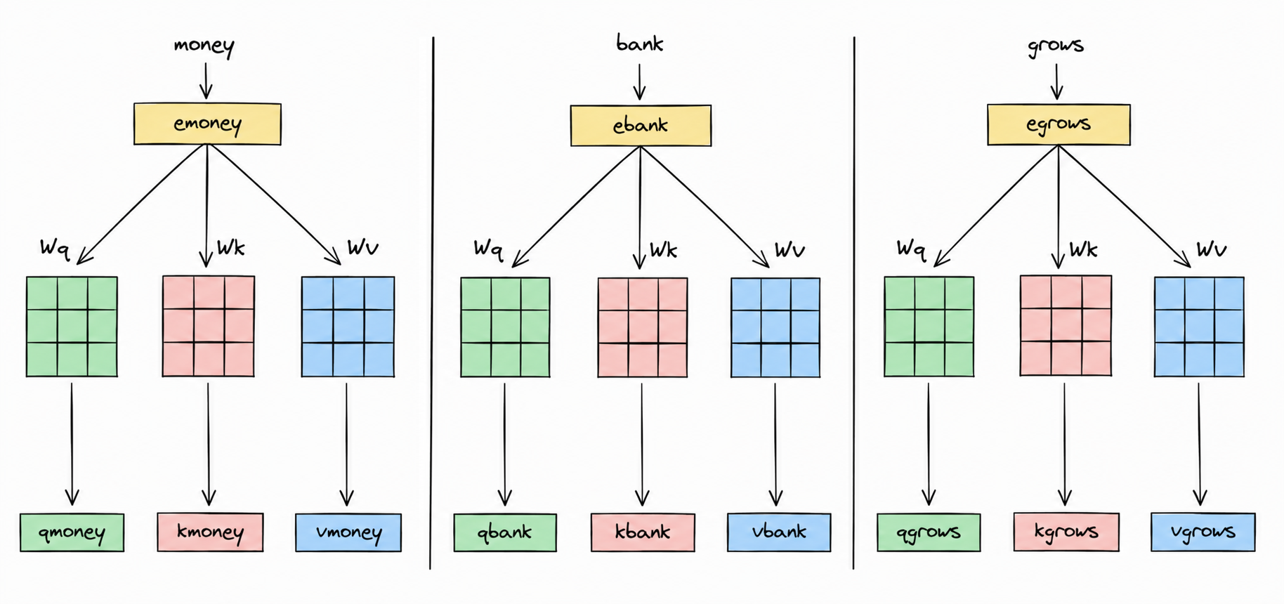
The following diagram illustrates this projection happening for every word in our sentence. Each embedding feeds into its own , , and matrices to produce its own Q, K, and V vectors:
Even more importantly, the matrices , , and are learnable parameters.
During training, the model can adjust these matrices to discover better Query, Key, and Value representations for the task at hand.
And this is precisely where learning enters the self-attention mechanism.
Where Do These Matrices Come From?
At this point, an obvious question arises.
Where do these matrices , , and come from?
More specifically, how do we determine the values inside these matrices?
Well, the answer is actually quite straightforward.
We are dealing with a deep learning model.
And just like most other deep learning architectures, we do not manually specify the values of these matrices. Instead, we initialize them with random values and allow the model to learn the appropriate values during training.
Initially, the matrices , , and contain nothing more than random weights.
As training progresses, the model makes predictions, computes an error, and uses backpropagation to determine how these weights should be adjusted.
Over many iterations, the matrices gradually evolve from random transformations into meaningful transformations that help the model solve the task it is being trained for.
In practice, these matrices are updated through gradient descent alongside all other trainable parameters in the network. Over time, they learn to project embeddings into representations that are increasingly useful for the task being optimized.
Eventually, assuming successful training, the model converges towards a set of weights that produce useful Query, Key, and Value representations.
The projection matrices are shared across all tokens in the sequence rather than being learned separately for each word. A single , , and produce every token's Query, Key, and Value vectors, which keeps the mechanism both trainable and highly scalable.
Even better, introducing these learnable matrices does not sacrifice the parallel nature of the architecture.
Once the embeddings have been assembled into a matrix, all Query vectors can be generated simultaneously through a single matrix multiplication.
The same is true for the Key vectors and the Value vectors.
In other words, despite becoming trainable, the architecture still retains one of its biggest strengths: all computations can be performed in parallel.
This ability to combine learnability with parallelism is one of the key reasons why Transformer-based architectures became so successful.
Applying This to the Full Sentence
Now, there is one very important detail that you should pay close attention to.
The matrices , , and are trained so that they learn how to generate the best possible Query, Key, and Value vectors from a given embedding vector.
In other words, after training, these matrices become capable of extracting the information most useful for querying, matching, and information aggregation.
One last thing.
Everything we just did for the embedding of bank must also be done for every other word in the sentence.
Consider our running example:
Money bank grows
First, we obtain the embedding vectors:
Now, for each embedding vector, we need three new vectors:
- a Query vector,
- a Key vector,
- and a Value vector.
For example, for the word money:
The exact same process is then repeated for bank:
And similarly for grows:
However, there is something very important that often confuses people when they first encounter self-attention.
The matrices used for money, bank, and grows are not different matrices.
The used for money is exactly the same used for bank.
Likewise, the used for bank is exactly the same used for grows.
The same is true for and .
Every word in the sequence uses the exact same Query, Key, and Value projection matrices.
The numbers inside those matrices are identical regardless of which word is being processed.
The only thing that changes is the input embedding.
As a result, starting from the three embedding vectors
we obtain a total of nine vectors:
And once we have these Query, Key, and Value vectors, the remaining procedure is exactly the same as the mechanism we developed earlier.
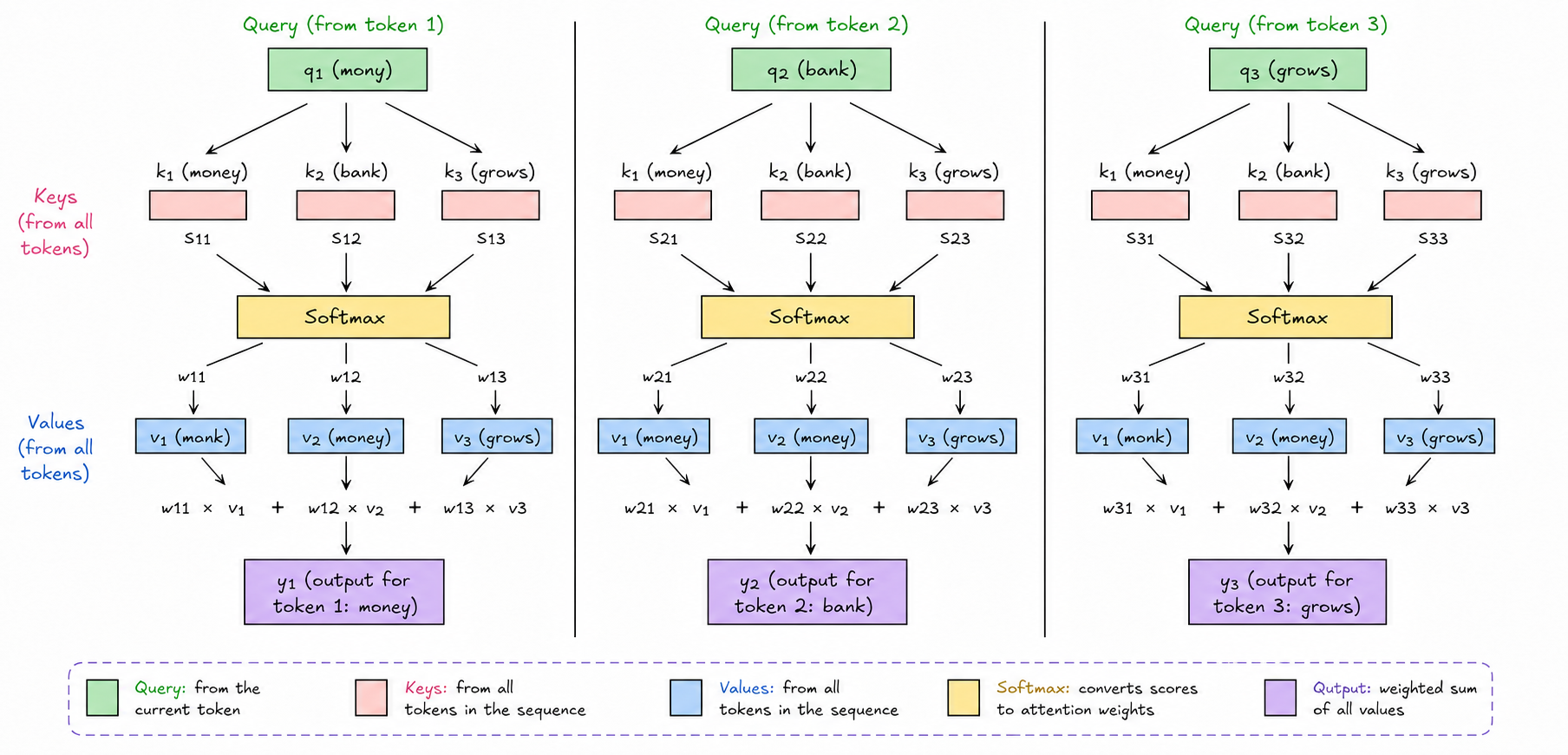
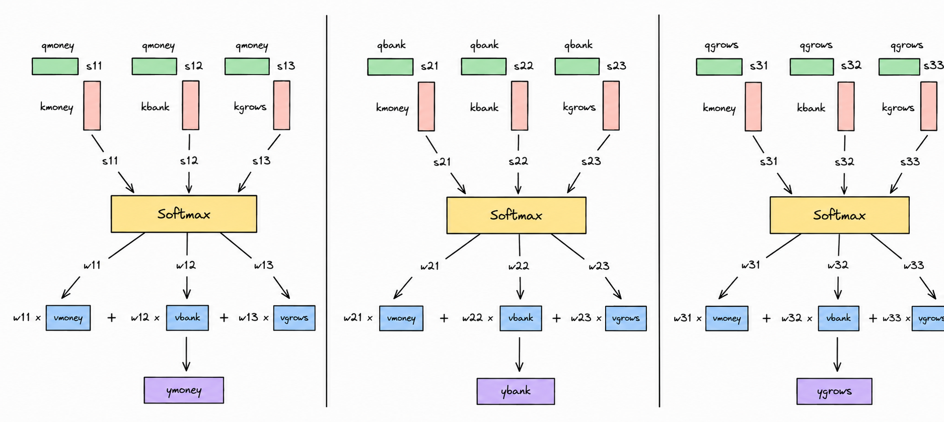
We compute similarity scores, normalize them using Softmax to obtain attention weights, and then use those weights to compute weighted sums of the Value vectors, ultimately producing the contextualized representations for each word. The following diagram illustrates exactly this for each word's Query vector against every Key vector in the sentence, followed by a weighted combination of the Value vectors:
And that's it.
What we have just built is the self-attention mechanism.
In fact, this is fundamentally the same self-attention mechanism that is used inside modern Transformer architectures today.
The process is straightforward:
- Start with the embedding vectors.
- Generate the corresponding Query, Key, and Value vectors.
- Use those Query, Key, and Value vectors to compute attention scores.
- Convert those scores into attention weights using Softmax.
- Use the attention weights to compute weighted sums of the Value vectors.
- Obtain contextualized representations as the final output.
Most importantly, because the Query, Key, and Value transformations are learned from data, the resulting representations are no longer merely general-purpose contextualized representations. Instead, they become representations shaped by the training objective, adapted through optimization to capture whatever patterns the data and the objective reward, which is exactly what we set out to achieve in the first place.
The Matrix Formulation
Everything we have discussed so far can also be represented as a single matrix computation, and this is in fact how self-attention is implemented in practice.
Instead of processing every word individually, we stack all embedding vectors together into a single embedding matrix , then multiply it three times using our three learnable projection matrices:
To make the dimensions explicit, using standard notation where denotes the number of tokens in the sequence, denotes the dimensionality of the input embeddings, denotes the dimensionality of the Query and Key vectors, and denotes the dimensionality of the Value vectors:
The matrix contains all Query vectors, contains all Key vectors, and contains all Value vectors, all generated simultaneously through matrix multiplication. This is the first place where the highly parallel nature of self-attention becomes clearly visible.
In modern Transformer implementations, the dimensionality of Query and Key vectors () is often chosen to be the same so that similarity scores can be computed using dot products. The Value vectors may use a different dimensionality () depending on the architecture, which is why separate notation is used for each.
Recall that for every word, we computed dot products between its Query and the Key of every other word to obtain a similarity score. At the matrix level, all of these scores are produced at once by multiplying with :
This single matrix automatically contains every pairwise similarity score we previously computed individually:
We then apply the Softmax function to convert these raw scores into normalized attention weights:
Softmax is applied row by row, not to the entire matrix at once: each row of holds one token's similarity scores against every other token, and after Softmax each row becomes its own probability distribution summing to 1. That is, it tells us how much attention one token pays to every other token. Each row therefore represents how a single token distributes its attention across every token in the sequence.
Before applying Softmax, however, the original Transformer paper introduces one more step. As embedding vectors grow larger in dimensionality, dot products grow larger in magnitude too, since they accumulate contributions across more dimensions. When the scores become very large, Softmax can become overly peaked, pushing nearly all the probability mass onto a single token and shrinking gradients enough to destabilize training. To counteract this, the scores are divided by before Softmax is applied, which keeps them in a more moderate range and the resulting attention weights spread more smoothly.
Let us call the resulting matrix of normalized attention weights , to keep it clearly distinct from the projection matrices , , and :
The complete, correct formulation is therefore:
This is the scaled dot-product attention formula from the original Transformer paper, and it is precisely what is used in modern implementations. The result is a matrix containing the contextualized representations for every word in the sequence.
The following diagram illustrates the entire pipeline together. The embedding matrix branches into , , and through their respective projection matrices. The similarity matrix is divided by , the row-wise Softmax normalization produces the attention matrix , and finally the weighted combination with yields the contextualized representations:
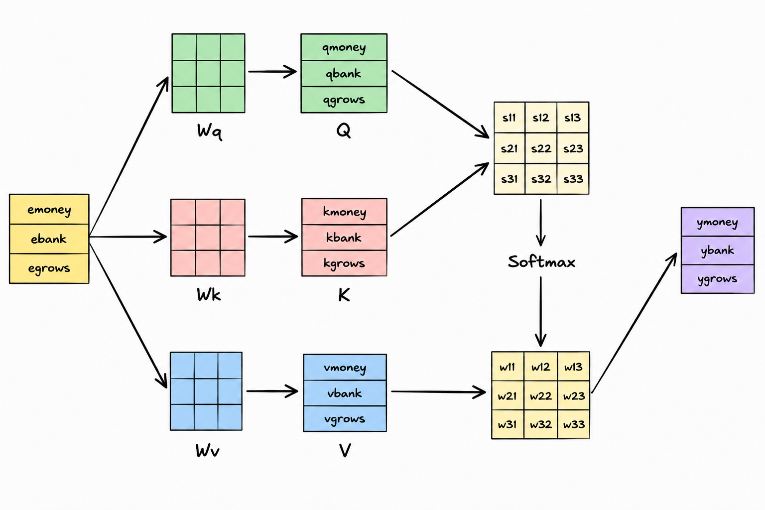
This matrix form does exactly what the word-by-word derivation did earlier; it is simply a more compact and computationally efficient way of expressing the same mechanism. Because the entire computation is expressed using matrix operations, modern hardware such as GPUs can execute it extremely efficiently in parallel, making Transformers both powerful and scalable.
Why This Matters for Training, Not Just Inference
The parallelism we identified in Observation 1 is not just a nice property at inference time. It is precisely what makes training Transformers at scale feasible in the first place.
Recurrent architectures process a sequence one token at a time: the computation for token 5 depends on token 4, which depends on token 3, and so on. Even during training, the model has to crawl through a sequence step by step, and on corpora containing billions of tokens, this becomes a serious bottleneck.
Self-attention removes it entirely. Because , , and are computed through simple matrix multiplications of , and because and are themselves just matrix operations, an entire batch of sequences can be pushed through the layer in one shot. Gradients for every token in every sequence can therefore be computed simultaneously rather than one token at a time, letting GPUs (built specifically for large matrix multiplications) be used to their full potential.
This is a big part of why Transformer-based models could be scaled to billions of parameters and trained on internet-scale datasets in a way that was simply not practical with recurrent architectures. Parallelism is one of the central reasons the Transformer revolution happened at all.
Conclusion
Let us take a step back and look at where we started.
The problem began with static embeddings.
A word such as Apple or bank would always receive the same vector representation regardless of the context in which it appeared. This made it difficult for models to distinguish between different meanings of the same word.
What we needed was a mechanism capable of producing contextualized representations.
And that is exactly what self-attention gives us.
Rather than treating a word in isolation, self-attention allows every word to gather information from every other word in the sentence. The result is a new representation whose meaning is influenced not only by the word itself, but also by the context surrounding it.
We then took this idea one step further.
By introducing Query, Key, and Value vectors, along with the learnable matrices , , and , we transformed a simple contextualization mechanism into a trainable architecture capable of learning task-specific representations from data.
Finally, by expressing the entire computation in terms of matrix operations, we obtained a mechanism that is not only powerful, but also highly parallelizable and computationally efficient, a property that turned out to matter just as much during training as it does during inference.
At first glance, the self-attention equation
may look intimidating.
However, as we have seen throughout this blog, behind that compact equation lies a surprisingly intuitive idea:
Every word looks at every other word, decides how important they are, and then uses that information to build a better representation of itself.
That simple idea is the foundation of the Transformer architecture and, consequently, the foundation of nearly every modern large language model we use today.
Go back to the very beginning of this blog, to the word Apple and the 10,000 sentences pulling its meaning toward a fruit, or to bank meaning two entirely different things in two entirely different phrases. Both were really the same problem: a representation that is fixed cannot serve a meaning that is fluid. Static embeddings froze a word's meaning in place the moment training ended; self-attention lets that meaning move, recomputed sentence by sentence from whatever words happen to be standing nearby. That single shift, from a fixed lookup table of meanings to something read in context, the way a person actually reads it, is why self-attention became the foundation the Transformer was built on, and why nearly every large language model in use today still traces its core computation back to the same scaled dot product between a Query and a Key.
And it all started with a simple question:
What if the representation of a word could adapt itself based on the words around it?
Self-attention is the mechanism that makes that possible, and now you know, from first principles, exactly how.
Epilogue: Why Self-Attention Is Not Always Enough
If you have made it this far, I believe you must have developed a fairly solid understanding of what self-attention is and how it works.
Read this final section as an epilogue to the article.
Based on everything we have discussed so far, self-attention appears to be the perfect solution to all of our embedding-related problems.
And it is.
For the most part.
Why for the most part?
Because, as it turns out, self-attention has a limitation of its own.
The mechanism works exceptionally well for sentences whose meaning can be understood through a single, clear interpretation. In such cases, self-attention is often able to gather the relevant contextual information and construct highly effective contextualized representations.
However, things become more interesting when a sentence can be interpreted from multiple perspectives.
As soon as self-attention encounters an ambiguous sentence, the quality of the representations it produces can begin to degrade.
You might be wondering:
What exactly is an ambiguous sentence?
Consider the following example:
The man saw an astronomer with a telescope.
Anyone with a basic understanding of English can interpret this sentence in at least two different ways.
The first interpretation is that there was a man who used a telescope to observe an astronomer.
The second interpretation is that there was a man who saw an astronomer who happened to be carrying a telescope.
Did you notice the issue?
Neither interpretation is incorrect.
Neither interpretation is more valid than the other.
Both are perfectly reasonable readings of the same sentence.
And that is precisely where the problem begins.
As humans, we can effortlessly construct multiple interpretations from a single piece of text. We can keep several possible meanings in our minds simultaneously and use additional context, if available, to decide which interpretation is most likely.
Machines, however, are not naturally equipped with this ability.
When a sentence admits multiple valid interpretations, a single self-attention mechanism has only one set of Query, Key, and Value projections through which it can analyze the sentence. As a result, it is forced to compress all of its understanding into a single attention pattern.
This does not mean that the model completely loses one interpretation. Rather, it means that the mechanism is limited in how many different relationships it can focus on simultaneously. Some relationships may end up receiving more emphasis, while others receive less.
A More General Perspective
The ambiguity example above provides an intuitive way to think about why a single attention mechanism might not always be sufficient. However, the motivation for using multiple attention heads is broader than ambiguity alone.
A single attention head is often sufficient to capture some important relationships within a sentence. However, language contains many different kinds of relationships simultaneously: syntactic relationships, semantic relationships, long-range dependencies, coreferences, positional patterns, and more.
While a single attention head can learn some of these patterns, it must represent everything through a single set of Query, Key, and Value projections. This limits the variety of relationships it can model at the same time.
As sentences become more complex, it becomes useful for different attention mechanisms to specialize in different types of relationships and representation subspaces.
You can think of the ambiguity example as one particular situation where multiple perspectives may be useful. More generally, multiple attention heads give the model additional flexibility to learn different ways of interpreting and relating tokens within the same sequence.
As sentences become more complex, this limitation becomes increasingly important.
So what is the solution?
Let us think about it intuitively.
Suppose a single self-attention mechanism is capable of focusing on one particular set of relationships within a sentence.
Then why not use multiple self-attention mechanisms at the same time?
Going back to our example, imagine having two independent self-attention blocks processing the same sentence simultaneously.
One might focus more heavily on the relationship between man and telescope.
Another might focus more heavily on the relationship between astronomer and telescope.
Each mechanism would be free to develop its own perspective on the sentence.
And when all of these perspectives are combined together, we obtain a richer representation than any single self-attention mechanism could produce on its own.
Bingo.
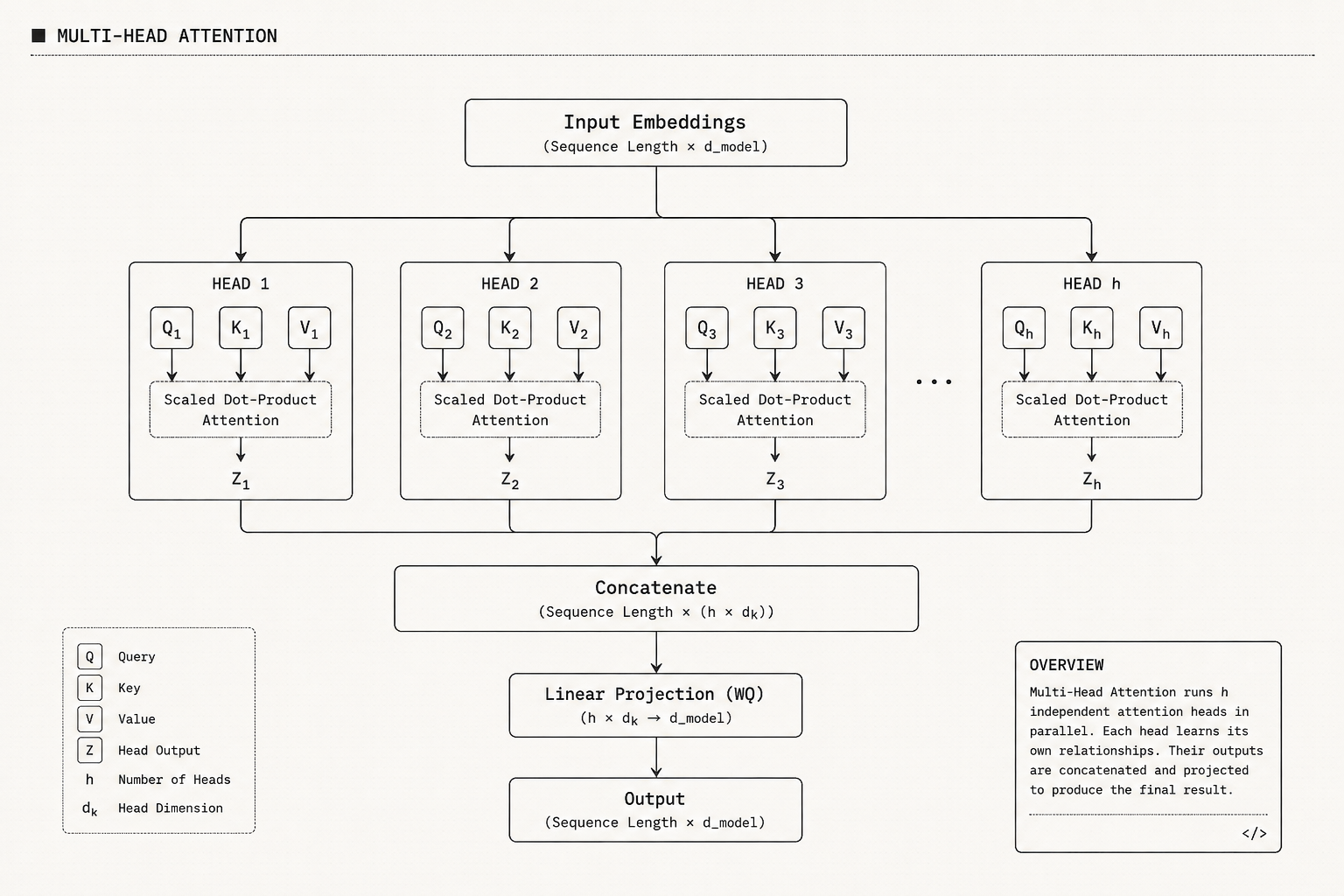
The idea we just arrived at is exactly what the industry calls Multi-Head Attention.
In other words, instead of relying on a single self-attention mechanism, we use multiple self-attention mechanisms simultaneously. Each of these mechanisms is free to learn its own attention patterns and focus on its own set of relationships within the sentence. Collectively, this allows the model to capture multiple perspectives that may be present in the same piece of text, producing richer and more expressive contextualized representations than a single attention mechanism could produce on its own.
Making the Idea Concrete
Let us make this idea more concrete with a simpler example.
Rather than working with a full sentence, let us consider the phrase:
Money bank
The phrase is intentionally simple because it allows us to focus entirely on the core idea behind multi-head attention without getting distracted by too many tokens.
Suppose we feed this phrase into two independent self-attention mechanisms, which we will call Head 1 and Head 2.
Even though both heads receive the exact same input embeddings, they do not share the same projection matrices.
Head 1 has its own:
while Head 2 has its own:
Because the projection matrices are different, the two heads are free to learn entirely different ways of looking at the same phrase.
One head might learn to focus heavily on the financial relationship between money and bank.
Another head might learn a different pattern altogether.
Both heads are observing the same input, but each is free to develop its own perspective.
And that is the central idea behind multi-head attention.
Applying Self-Attention — Head by Head
Now, we already understand how self-attention works. So rather than introducing an entirely new mechanism, let us simply apply everything we already know to this example.
Recall our phrase:
Money bank
The first step remains exactly the same.
We begin by generating embedding vectors for the two words:
At this stage, these are simply the input embeddings that will be fed into the attention mechanism.
Next, just as we did in the self-attention section, we project these embeddings into Query, Key, and Value spaces using linear transformations.
In ordinary self-attention, this is accomplished using a single set of projection matrices:
which produce one Query vector, one Key vector, and one Value vector for each word.
Since we have two words, we obtain:
and
for a total of six vectors.
So far, everything is identical to the self-attention mechanism we developed earlier.
Now comes the important difference.
Suppose we decide to use two attention heads instead of one. Since each head is intended to learn its own perspective on the input, each head must have its own independent set of projection matrices.
Head 1 therefore has:
while Head 2 has:
Notice what has happened. The number of projection matrices has doubled. And because each set of projection matrices generates its own Query, Key, and Value vectors, the number of intermediate vectors doubles as well.
For the word money, we now obtain:
and
Similarly, for the word bank, we obtain:
and
In total, we now have twelve Query, Key, and Value vectors instead of six.
Each attention head then performs its own self-attention computation independently.
Head 1 produces its own contextualized representations:
while Head 2 produces:
Instead of obtaining a single contextualized representation for each word, we now obtain multiple contextualized representations — one from each attention head. And because each head has learned its own Query, Key, and Value projections, each head is free to focus on different relationships within the same input sequence.
The Attention Computation — Nothing New Here
At this point, nothing fundamentally new is happening. Each head simply performs the exact same self-attention computation that we studied throughout this article.
For each head, we:
- Compute the Query-Key similarity scores using dot products.
- Scale those scores by .
- Pass the scaled scores through the Softmax function to obtain attention weights.
- Use those attention weights to compute weighted combinations of the Value vectors.
In other words, each head independently computes:
For Head 1, this produces:
Likewise, Head 2 performs the same computation using its own Query, Key, and Value vectors, producing:
Notice the key difference from ordinary self-attention.
With a single attention head, each word receives a single contextualized representation.
With two attention heads, each word receives two contextualized representations — one from each head.
For example, instead of a single contextual embedding for bank:
we now obtain:
Similarly, instead of a single contextual embedding for money:
we now obtain:
Each of these representations captures the perspective learned by its respective attention head.
At this stage, we have successfully extracted multiple contextual views of the same input sequence. The only question that remains is:
How do we combine them into a single representation that can be passed to the next layer?
A Quick Note
Throughout this discussion, we used two attention heads purely for intuition and ease of understanding.
In practice, there is nothing special about the number two.
We can use any number of attention heads, allowing the model to learn multiple perspectives on the same input sequence simultaneously.
In fact, the original Transformer paper used 8 attention heads.
You can think of this as running eight independent self-attention mechanisms in parallel, each free to learn its own Query, Key, and Value projections and therefore its own way of interpreting the input.
Another important observation follows immediately from what we already know.
Earlier in this article, we saw that self-attention is highly parallelizable. Every token can compute its attention scores simultaneously, making the mechanism extremely efficient on modern hardware.
Multi-head attention preserves this property.
Even though we now have multiple attention heads, all of those heads can be computed in parallel as well. Each head performs its own attention calculation independently, allowing modern GPUs to process them simultaneously during training and inference.
For simplicity, we will not dive into the full matrix implementation here.
However, there is one final piece of the puzzle that we should understand.
Combining the Heads: Concatenation and the Output Projection
Recall that our two attention heads produced:
and
In other words, each head produced its own contextualized representation of every token.
The question is: how do we combine these multiple perspectives into a single representation?
The answer is surprisingly simple.
We concatenate the outputs of all attention heads together.
If we had two heads, we would concatenate the outputs from Head 1 and Head 2. If we had eight heads, we would concatenate the outputs from all eight heads. This produces a larger vector containing all learned perspectives side by side.
You might wonder why we concatenate rather than, say, average the outputs. The reason is that averaging would collapse the distinct perspectives each head learned into a single blended signal, losing the individual structure each head captured. Concatenation preserves all of that information and lets the next step — the output projection — decide how to combine it.
We multiply this concatenated representation by another trainable matrix:
often referred to as the output projection matrix.
The purpose of is not to select a single "correct" perspective. Instead, it learns how to combine the information gathered by all attention heads into a unified representation.
You can think of the attention heads as a group of specialists, each contributing its own interpretation of the input. The output projection matrix then learns how to blend those interpretations together into a final contextualized representation.
Mathematically, this operation is written as:
where denotes the number of attention heads.
A Small Detail About Dimensions
There is one subtle implementation detail worth mentioning.
The original Transformer architecture used:
meaning that every input embedding had dimensionality 512.
However, each of the 8 attention heads did not operate directly on 512-dimensional Query, Key, and Value vectors. Instead, the projection matrices reduced the dimensionality for each head:
Since there were 8 heads:
which means that after concatenating the outputs of all eight heads, we once again obtain a 512-dimensional representation.
This design significantly reduces computational cost because each individual attention head operates on much smaller vectors, while the concatenation step restores the full representational capacity of the model.
The projection matrices for each head therefore have the following shapes:
for each head .
Finally, the concatenated 512-dimensional representation is multiplied by:
to produce the final output of the multi-head attention block.
Notice something elegant here.
The dimensionality entering the multi-head attention block is the same as the dimensionality leaving it.
A 512-dimensional embedding enters the module. A 512-dimensional contextualized embedding leaves the module. Only the intermediate computations are performed in lower-dimensional spaces.
This allows the architecture to gain the benefits of multiple attention heads without increasing the dimensionality of the representations flowing through the network.
Closing Thoughts
And that, in essence, is multi-head attention.
Self-attention taught us how a word can gather information from the words around it.
Multi-head attention extends that idea by allowing multiple attention mechanisms to perform that gathering process simultaneously, each learning its own way of looking at the same input.
The result is a richer, more expressive representation than any single attention head could typically produce on its own.
Most importantly, notice how little actually changed.
We did not invent a new attention mechanism.
We did not replace self-attention.
We simply took the same self-attention mechanism that we spent this entire article building from first principles and ran it multiple times in parallel.
Sometimes, the most powerful ideas are not entirely new ideas.
They are simple ideas repeated in the right way.