The Encoder-Decoder Architecture: Building Sequence-to-Sequence models

For the longest time, NLP problems involving variable length input-output sequences used to be tackled with the help of unidirectional and bidirectional LSTMs, GRUs and RNNs.
Then, researchers introduced a new architecture to deal with these sequence-to-sequence problems, problems with variable length inputs and outputs. They tested their newly designed architecture on a machine translation task from English to French, and they broke the curve by achieving a BLEU score higher than the state of the art at that time.
We will get to what exactly they proposed, but let's just understand what exactly we are dealing with right now, what could be a task involving variable length input and output.
A prominent example of such a task would be machine translation, i.e., language translation, translating text from one language to another.
In our examples throughout this blog, we will be taking the task of English to Hindi machine translation. So our input would be English and output would be Hindi.
The Dataset
To train an architecture on such tasks, there are specialized datasets available. Basically, you have two columns, one of the source language and another of the destination language, the language you want to translate the text into.
For this running example, we are going to take a small dataset of just two rows:
| English | Hindi |
|---|---|
| Think about it | सोच लो |
| Come in | अंदर आ जाओ |
So now we have the dataset, and we know the problem we are dealing with. Now let's come to the architecture.
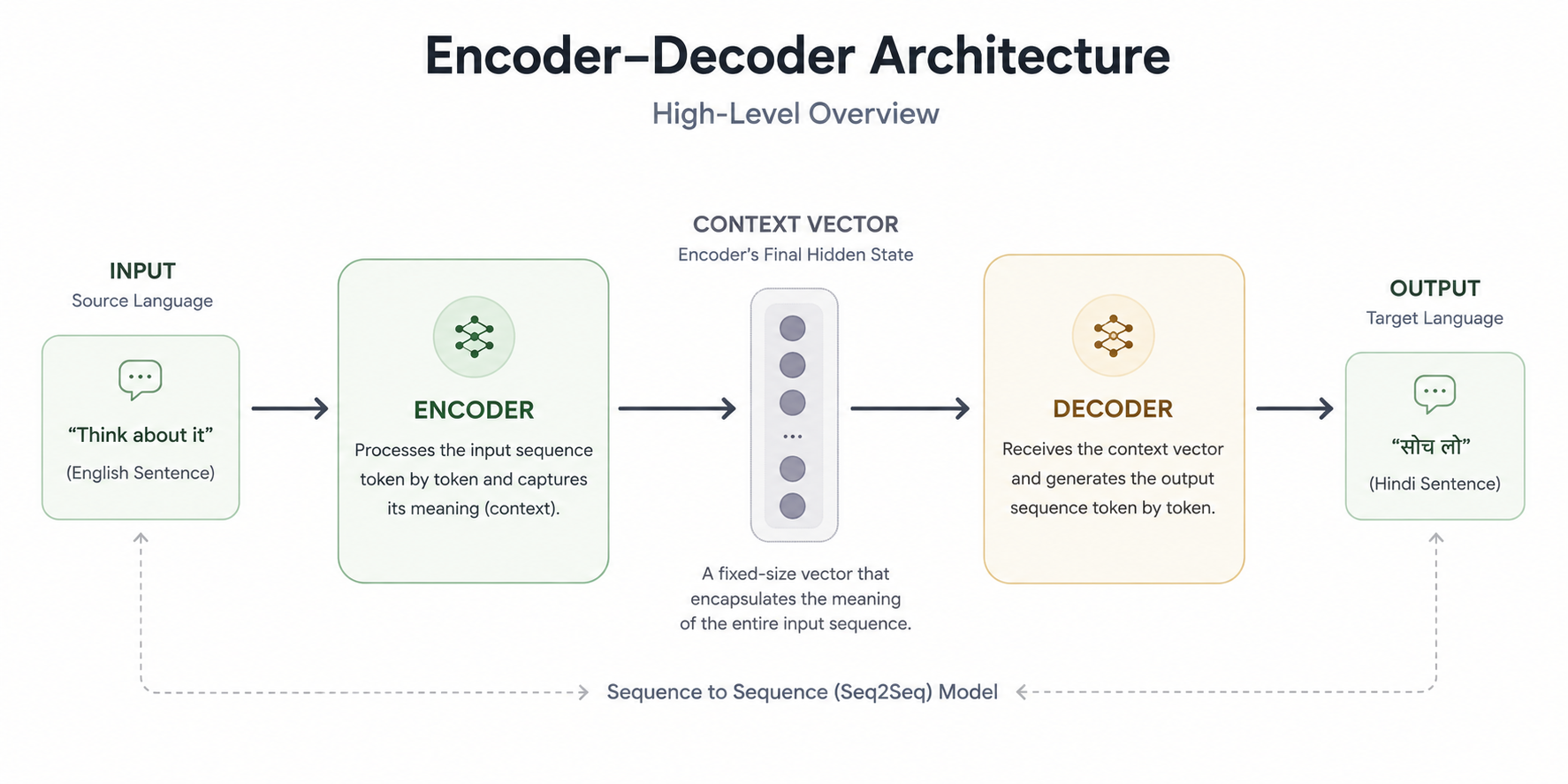
High-Level Architecture
The high-level overview of this architecture is very simple. It can be understood by a kid, even. We have three things.
1. Encoder
The encoder takes input from the user, and it takes input in a sequential manner, token by token (you can say word by word, but token by token is more accurate). It tries to capture the meaning of each token and carries forward that captured meaning. It tries to understand the context of the word, of the token.
When it does that for the whole sequence, the whole sentence, by the time the encoder has processed one example or one data point from the dataset, it has generated something called a context vector, basically its final hidden state (and cell state for LSTMs).
2. Context Vector
A context vector is nothing but the semantic meaning, it is just the essence of what the sentence inputted into the encoder is trying to deliver, in vectorized format. A vector is nothing but a set of numbers.
To be more precise, the context vector is simply the encoder's final hidden state (and cell state for LSTMs) at the last time step. By the time the encoder has processed every token in the input sentence, these final states are passed to the decoder as the context vector.
Now, here's a small caveat worth keeping in mind: this context vector is the encoder's attempt to squeeze the meaning of the entire input sentence into one fixed-size vector. For short sentences like ours, that's fine. But for long sentences, cramming everything into this single vector becomes a bottleneck, the encoder just doesn't have enough room to hold on to all the details. This is one of the main motivations behind attention, which we'll get into in the later blogs.
3. Decoder
You can assume this decoder to be very similar to the encoder. It is just that this decoder receives the context vector as input and tries to convert this context vector into human-readable language in the target language.
So, to get the idea straight: the encoder takes the source language, processes it, and converts it into a context vector. That context vector goes to the decoder, the decoder understands the context vector, and processes it again to output human-readable text in the target language.
This is a high-level overview of what this encoder-decoder architecture is.
What's Under the Hood?
Under the hood, the encoder and decoder are nothing but LSTM cells or GRU cells. We do not use plain RNNs because they have the vanishing gradient problem. The researchers in the original paper used LSTMs.
Preparing the Data: Tokenization and Vocabulary
Given that we understand the architecture from a high level, let's get into the training of this system. Let's expand the encoder, let's unfold it, and let's do the same for the decoder.
Coming back to our dataset, remember, our dataset had two rows. Let's tokenize our dataset and make vocabularies out of them.
For the English side, it would be a five-word vocabulary:
think, about, it, come, in
Now, the simplest way of representing each word uniquely in this five-word vocabulary is through one-hot encoding. We take a five-dimensional vector, and for each word, the position assigned to that word is marked as 1 while all the remaining positions are set to 0. This gives every word a unique representation.
So for "think", it would be:
think → [1, 0, 0, 0, 0]
Similarly, for all the others, and assuming "in" is the last word of the vocabulary:
in → [0, 0, 0, 0, 1]
And that is how it would go for all the other words in the English vocabulary.
Now let's come to the Hindi vocabulary. Ideally, this Hindi vocabulary also has five words: सोच, लो, अंदर, आ, जाओ, but since this is the target language, we need two additional words in it. These words are special symbols: the <start> token and the <end> token.
These are really important as they signal the decoder when to start generating the output and when to stop generating the output. As soon as the decoder sees the start token, it starts generating the output. As soon as it sees the end token, it stops generating the output.
So we are going to one-hot encode this as well, but now the Hindi vocabulary is not of five words, but of seven words.
Unfolding the Encoder
The encoder is nothing but a bunch of LSTM cells connected to each other sequentially.
As you already know, an LSTM maintains two states: the hidden state and the cell state. At the beginning of the encoding process, these states are typically initialized to zeros, although some implementations use learned initial states instead. The first token, "think", is then fed into the encoder together with these initial hidden and cell state values.
The LSTM cells process the input sequence one time step at a time. At the first time step, we feed the token "think" into the encoder. At the second time step, we feed "about", at the third time step "it", and so on.
At each time step, the LSTM receives the current input token along with the hidden state and cell state from the previous time step. Based on the standard LSTM update equations, these states are updated and passed on to the next time step. We will not go into the details of those updates here.
Now, when we say that "think", "about", or "it" is going as input, it is not the words themselves that are going in, it is the one-hot encoded versions of them.
Encoder input sequence:
think → about → it
The context vector for the decoder is nothing but the last and final LSTM cell's final hidden state (and cell state for LSTMs) from the encoder.
Unfolding the Decoder
Now let's come to the decoder. As we already talked about, the decoder is also LSTM, so its initial cell state and hidden state values will be exactly the encoder's final hidden state (and cell state for LSTMs), which is nothing but the context vector.
We send the first token for the decoder, and the first token is the start token.
Decoder initial state = Encoder's final context vector
Decoder first input = <START>
Here is the interesting bit: we make sure to attach a softmax layer on top of every cell of the decoder LSTM. Why? Because this softmax layer builds out probabilities, it spits out probabilities for what the next token in the target sentence should be, given the context vector and everything the decoder has generated so far.
Very important: the number of units in this softmax layer will be exactly equal to the number of words in the decoder vocabulary, seven, in our case.
Now, assuming we gave the context vector and the <start> token to the decoder, and this softmax layer generated some probabilities. Let's say the second parameter got the highest value. Based on the probabilities generated by the softmax layer, the output comes out to be "लो". But for "think", the actual translated output should have been "सोच".
Decoder step 1:
Input: <START>
Predicted output: लो
Expected output: सोच
This means our model is not learning yet, which is obvious because we just started training.
Teacher Forcing
Here is the catch: if we send this output of the LSTM cell as the input for the next LSTM cell, we can do that, but early on in training, this output is often wrong, and if we feed that wrong output forward, the mistake just keeps propagating to the next timesteps and the next, throwing everything off down the line. So the workaround is something called teacher forcing.
The idea is pretty simple. Regardless of whatever is generated as the output of the current LSTM cell in the decoder, the input for the next LSTM cell will always be the ground-truth target token from the dataset, i.e., the actual correct token that was supposed to appear at that position in the target sequence.
So even though the LSTM generated "लो" as the output, we will send "सोच" as the correct input for the next LSTM cell.
Decoder step 2:
Input (teacher-forced): सोच
Predicted output: लो (correct, by chance)
This is teacher forcing, regardless of whatever output comes, we always feed the ground-truth target token from the dataset as the next time step's input.
Remember, this teacher forcing step is done only during the training phase, not while predicting. If we did this during prediction, it would defeat the entire purpose.
So during training, you send the correct one-hot encoding of what the dataset says the translation should be.
Training vs Prediction
Before we move on, here's a quick side-by-side so the difference is clear:
| Aspect | Training | Prediction |
|---|---|---|
| Mechanism used | Teacher forcing | Model-generated outputs |
| Next decoder input | The correct token from the dataset | The model's own previous prediction |
| Purpose | Speeds up and stabilizes learning | Reflects how the model actually behaves at inference time |
Walking Through the Full Decoding Sequence
So for "think about it":
Time step 1: input is
<START>, the softmax gives some probabilities, and an output gets generated. It was wrong ("लो" instead of "सोच"), so in the next time step, even though the output was wrong, we send the correct input ("सोच"). Gradually, this system will start to learn.Time step 2: we send the token "सोच", and let's assume the LSTM cell outputs "लो", which is the correct translation according to our dataset.
Time step 3: when we send "लो" as input, the LSTM cell outputs the
<END>token.
Decoder sequence (training, with teacher forcing):
<START> → सोच → लो → <END>
Now, here is where it gets interesting. During inference, the decoder stops as soon as it predicts the <END> token, because the end token signifies that the translation is complete.
Calculating the Loss
Now, we will look at the actual true translation for "think about it" from the dataset, which is "सोच लो", and we will compare it with the translation the model actually generated.
Expected:  सोच → लो → <END>
Predicted: लो → लो → <END>
The first "लो" was a mistranslation, it should have been "सोच".
So here's how the loss actually gets calculated. At every single decoder timestep, we compare the predicted probabilities against the actual correct token for that timestep, and we calculate the categorical cross entropy loss for that one prediction. So for "think about it", we get one loss value for the first timestep (predicted "लो", actual "सोच"), another loss value for the second timestep (predicted "लो", actual "लो"), and another loss value for the third timestep where the actual token is <END> (and the prediction was also <END> here, so this one contributes a small loss).
Since we have a fixed vocabulary, this is a categorical task, so the loss function at each timestep is categorical cross entropy:
Here, is the one-hot encoded target, so only the term where (i.e., the correct token) survives the sum, meaning the loss at each timestep is simply the negative log of the probability the model assigned to the correct token.
Once we have these individual, per-token losses for the whole sequence, we sum them up (or take their average) to get a single loss value for that sequence.
If we are training with batches, we then average these sequence losses across all examples in the batch to obtain a single batch loss.
Forward Propagation and Backpropagation
Once we have passed a batch of input sentences through the encoder, run the decoder, and calculated the batch loss, we can say one forward propagation pass is complete.
The next step is backpropagation. We have calculated the loss, and now we try to minimize it, that's the standard approach in deep learning.
Now, when we backpropagate, the gradients flow backward through all the decoder timesteps, through the context vector, and then through all the encoder timesteps too. This whole process of running gradients backward through time like this has a name, it's called Backpropagation Through Time, or BPTT for short.
And here's the neat part: the gradients coming from the decoder don't just stop at the decoder, they flow through the context vector and continue right into the encoder. So both the encoder and the decoder end up learning together, as one connected system.
For backpropagation, we calculate the gradients, and then we run an optimizer, it can be SGD, Adam, RMSprop, or whichever you want.
You run the optimizer with a set learning rate, and you get updated weights for the whole architecture. Then you start forward propagation again.
This is how training is done, for however many epochs you might like.
Just a quick note on terminology before we move on: one iteration is basically one forward pass plus one backward pass over a single batch, that's it. An epoch, on the other hand, is when you've gone through your entire dataset once, batch by batch, doing this forward-backward thing for all of them. So if your dataset has, say, 10 batches, then 10 iterations make up one epoch.
Prediction
Now that our training is done, let's come to predicting. The prediction setup is very similar to training. The only difference is that we don't impose teacher forcing.
Whatever a particular LSTM cell in the decoder generates as output, we send that generated output as the input for the next LSTM cell in the decoder, instead of feeding it the "correct" answer from a dataset, since at prediction time we don't have one.
So at prediction time, it works like this:
Step 1:
Input: <START>
Context vector: from encoder
Output: सोच   (model's own prediction)

Step 2:
Input: सोच   (the model's own previous output, fed back in)
Output: लो

Step 3:
Input: लो   (the model's own previous output, fed back in)
Output: <END>

Final translation: सोच लो
The decoder keeps feeding its own previous prediction as the next input, time step after time step, until it predicts the <END> token, at which point it stops generating further output. This chaining of "output becomes input" is exactly what teacher forcing skips during training, and exactly what happens during prediction.
Improvements to the Architecture
We can make some improvements in this architecture to achieve better results.
1. Embeddings Instead of One-Hot Encoding
Instead of using one-hot encoding, we use an embedding layer. Why? Because in our example, we had a very small vocabulary. In real-world datasets, however, vocabularies can contain tens or even hundreds of thousands of words. Representing each word as a one-hot vector would be highly inefficient, since the vector would be extremely large while containing only a single non-zero value.
Instead, we map each token to a dense embedding vector of a fixed size, such as 128, 256, or 512 dimensions. Unlike one-hot vectors, embeddings can learn meaningful relationships between words and represent them in a much more compact form. This reduces memory usage, makes computations more efficient, and provides the model with richer representations of the input tokens.
2. Deep (Stacked) LSTMs or GRUs
Instead of using single-layer LSTMs or GRUs, we use deep/stacked LSTMs or GRUs, a three-layer or four-layer setup. The original paper used a four-layer LSTM setup.
When we use deep or stacked LSTMs/GRUs, it's not that each layer cleanly maps to "word level" or "sentence level" or "paragraph level", it's more nuanced than that, but there is a general trend worth knowing:
- Lower layers tend to learn more local patterns, things closer to the raw input.
- Higher layers tend to learn more abstract representations, capturing broader relationships across the sequence.
3. Reversing the Input Sequence
Instead of sending the input as "think about it", we send it as "it about think", we reverse the input given to the encoder.
This works well in some language pairs where the context is more dependent on the initial words, like English and French. How does it help? The distance between an input token in the encoder and the corresponding output token in the decoder for the same word becomes smaller, this shorter dependency path makes optimization easier, since gradients have less distance to travel between corresponding input and output tokens during backpropagation, so the model captures the semantic relationship better.
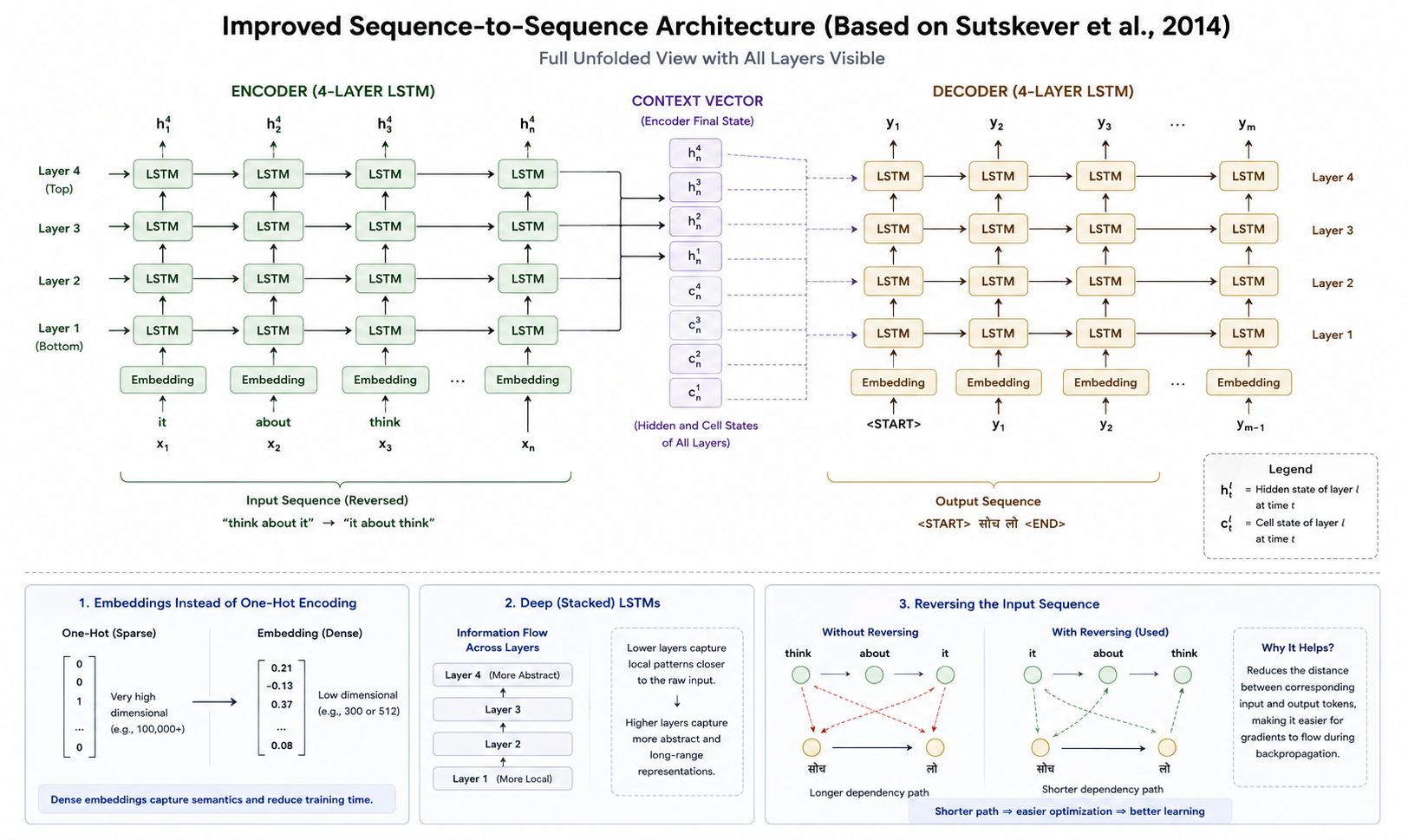
All three improvements mentioned above are exactly the ones used in the original paper, these were the exact architecture design elements used by the researchers when writing it.
Conclusion
So that's the encoder-decoder architecture for sequence-to-sequence tasks, an encoder that reads the input token by token and compresses it into a context vector, a decoder that takes that context vector and generates the output token by token, teacher forcing to speed up training, and a few key improvements like embeddings, stacked LSTMs, and input reversal that take this from a toy example to something close to what the original paper actually used.