Attention: Breaking the Seq2Seq Bottleneck

Before we begin, I am going to assume that you either have read my previous blog on encoder-decoder architectures or already have a decent understanding of how Seq2Seq models work. Everything we discuss in this blog builds directly on top of those ideas.

You can read it here↗.

Now, with that foundation in place, let's look at why the attention mechanism was needed in the first place.

Why do we even need attention?

You must be wondering, why do we even need a new mechanism or a new architecture when the encoder-decoder architecture solved the sequence-to-sequence problems? Example, summary generation, machine translation, etc.

Here is the answer. Although the encoder-decoder architecture works well on these kinds of tasks, its output quality starts to degrade the moment the sentence length increases, the moment the sentences become lengthy, let's say more than 30 words.

Why does this happen? This happens because of the context vector. Remember, we saw that the context vector is, in layman terms, the summary or the essence of the whole sentence that has been processed by the encoder, that is later fed to the decoder. Now what happens is, as the sentence length grows, the context vector starts failing in catching up with the nuanced or minute details in the long sentences, which is pretty obvious because if we want to summarize a whole paragraph in a fixed-size vector, it will lose its quality. It will lose details. So this is one issue, and this issue is from the encoder side.

There is another reason behind the need for a new and improved architecture, and that is from the decoder's side. It's not an issue, it's a reason. The reason is, different output words depend on different parts of the source sentence, not the whole input equally.

Let me explain it properly. Suppose we are dealing with a task of machine translation from English to Hindi. "Turn off the lights" is the source and "लाइट बंद करो" is the target. So this Hindi phrase "बंद करो" is only dependent on, or is only being translated from, "turn" and "off." "Light" has no relevance, or negligible relevance, in this case. So this is the thing from the decoder's side. Did you get it?

What is the solution? The solution is, at every time step of the decoder, we have to dynamically feed this information into the decoder: which encoder hidden states are important to generate the output at that given time step from the decoder. This mechanism is called the attention mechanism.

Building intuition with an example

Now, before we take a deep dive into the world of attention, let's take an example. Let's build intuition. We will carry forward throughout this blog, to make things more intuitive and to make sure that everything clicks.

The task is machine translation. We have a sentence in English, and we have to translate it into Hindi. The sentence is "turn off the lights." Its Hindi translation would be "लाइट बंद करो."

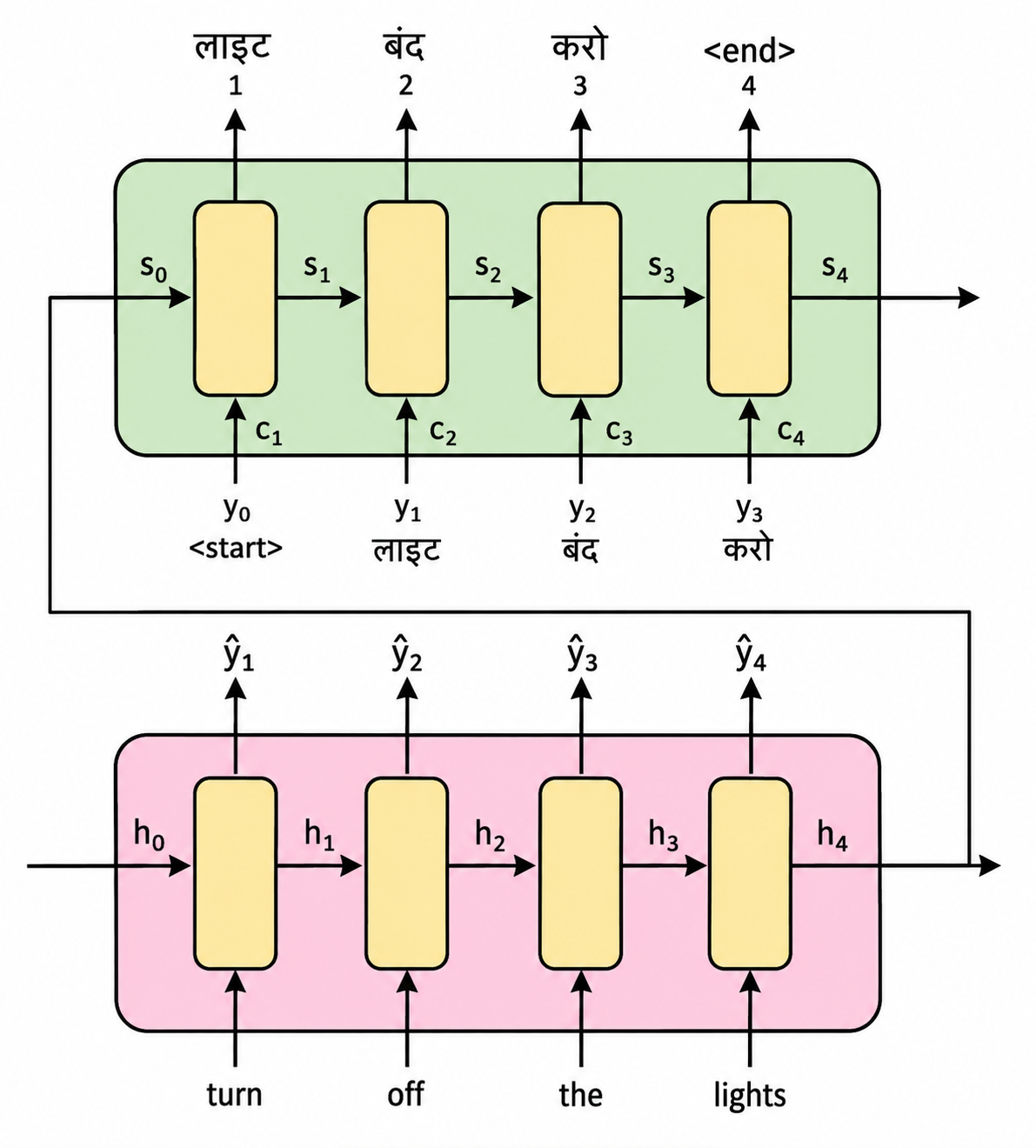
So, on the basis of what we know already, according to the encoder-decoder architecture, the setup would look something like this.

Setting up notation

Now, before we move forward, let us set some notation that will help us throughout this blog.

• $h_i$ is the $i^{th}$ hidden state of the encoder.
• $s_i$ is the hidden state of the decoder at decoder time step $i$.
• $y_i$ is the decoder input token at decoder time step $i$.
• $\hat{y}_i$ is the output token predicted by the decoder at decoder time step $i$.
• $c_i$ is the attention context vector computed for decoder step $i$.

At decoder step $i$, the decoder receives $y_{i-1}$ as input and produces the output token $\hat{y}_i$.

The key addition here is $c_i$, the attention context. You can see that, along with $y_i$ and $s_i$, the decoder now receives another input: $c_i$.

This $c_i$ is supplied at every decoding step and tells the decoder which parts of the input sequence are most relevant at that particular moment. In many ways, it is the heart of the attention mechanism.

So, to be precise, attention no longer relies on just that one fixed context vector for the entire decoding process. Instead, at every step, a fresh $c_i$ is computed and fed in, based on what the decoder thinks it needs at that particular moment.

You can think of $c_i$ as a custom summary of the input sentence, created specifically for the current step. It's not one summary for the whole sentence anymore. It's a new, tailored summary every single time the decoder is about to predict a word.

Calculating $c_i$

Let's see how this $c_i$ is computed. For any given time step $i$ of the decoder and $j$ of the encoder:

We already know that $h_j$ is the $j^{th}$ hidden state of the encoder. The new term here is this $\alpha_{ij}$. It is pretty important.

Now, where do these $\alpha_{ij}$'s actually come from? They come from a raw score, called the alignment score, $e_{ij}$, which then gets normalized into $\alpha_{ij}$. We'll get into exactly how in a bit, but just keep this in mind for now: $e_{ij}$ is the raw, unnormalized version, and $\alpha_{ij}$ is what you actually use as the weight.

This $e_{ij}$ depends on two things: $h_j$, which is the current encoder hidden state, and $s_{i-1}$, which is the previous hidden state of the decoder.

Now, you might be wondering: why does the alignment score depend on the previous hidden state of the decoder?

The reason is that translation is not performed one word at a time in isolation. When generating the output at decoder step $i$, the model must take into account everything it has produced so far. In other words, the question attention is trying to answer is:

Given the current state of the decoder, how useful is the $j^{th}$ encoder hidden state for generating the next output word?

This is why the alignment score depends not only on the encoder hidden state $h_j$, but also on the previous decoder hidden state $s_{i-1}$. The decoder's hidden state contains information about the translation generated up to that point, allowing attention to decide which parts of the input sentence are most relevant right now.

So, the next word produced by the decoder depends not only on the information coming from the encoder, but also on the context that the decoder has built throughout the translation process.

Back to our example

Let's look at our example to make this more concrete. Now we somewhat have an idea of how the newer architecture looks.

As you can see in the figure above, rather than relying on one fixed context vector throughout decoding, we compute a fresh $c_i$ at every step.

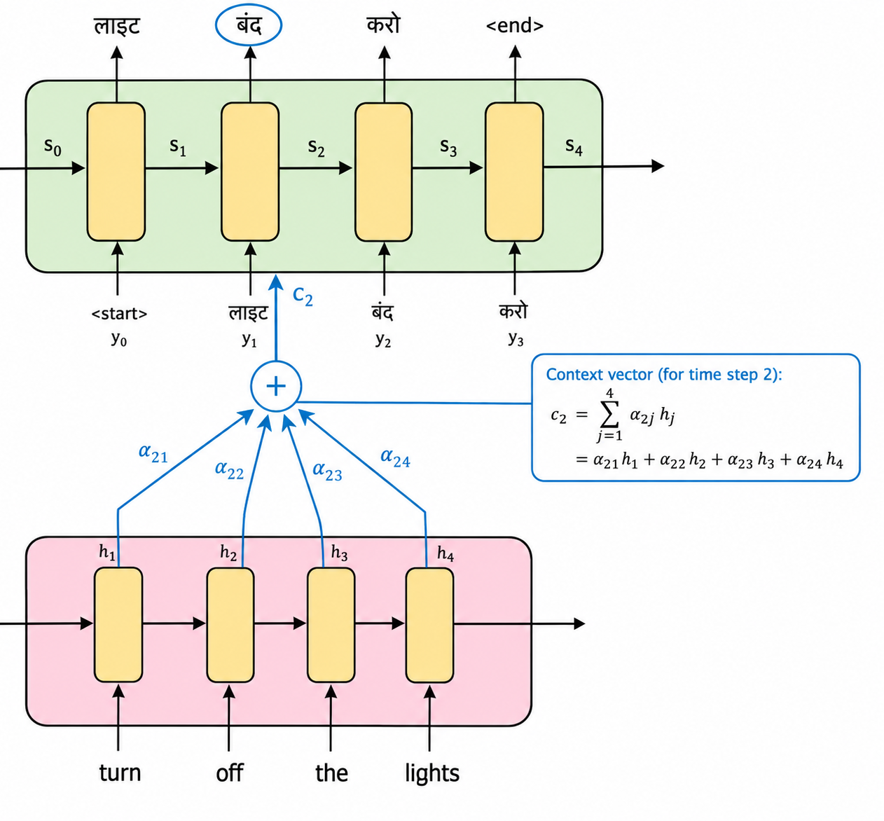
Now, assuming that we are on the second time step of the decoder, and "लाइट" has already been printed at $i-1$, we now have to predict the word at the second time step, given we already have "लाइट," the previous hidden state of the decoder, and all the hidden states of the encoder.

Let's calculate $c_2$. As we remember, $c_2$ will be the weighted sum of all the alphas, $\alpha_{2j}$, multiplied by $h_j$. That is:

And this weighted sum basically makes the $c_2$, which tells the decoder the role of every hidden state of the encoder in predicting the output of this second step.

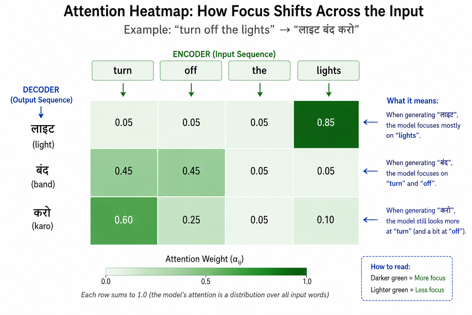
To make this even more intuitive, think about what the weights would roughly look like for our example. While generating "लाइट" (the first output word), the attention weights would probably look something like: "turn" gets a small weight, "off" gets a small weight, "the" gets a small weight, and "lights" gets a large weight, since "लाइट" is really being translated from "lights." Then, while generating "बंद," the weights would shift: "turn" and "off" would now get large weights, and "lights" would drop to a small weight, because "बंद" comes from "turn off," not from "lights." That's the whole point of attention. The weights aren't fixed, they move around depending on what the decoder is trying to produce right now.

Looking inside alpha

Till now, we have gained a good idea of what attention is. Now let's actually look inside that alpha. How exactly do you calculate it?

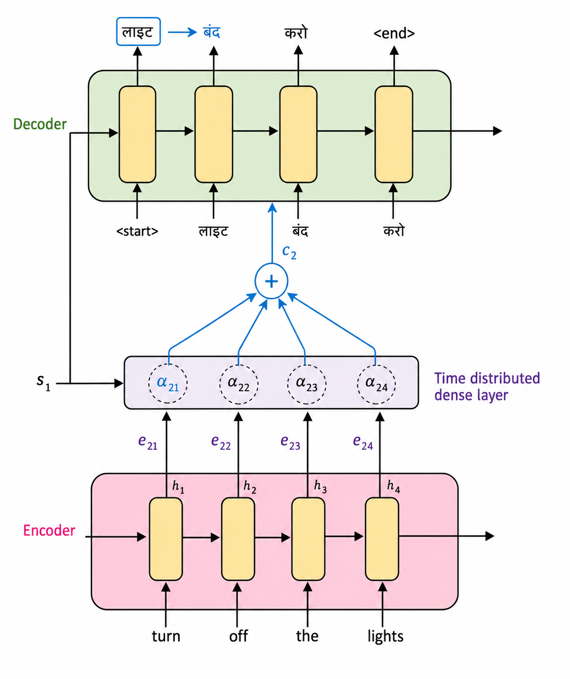
As we already discussed, the raw alignment score $e_{ij}$ is dependent on the $j^{th}$ hidden state of the encoder and the $s_{i-1}$ hidden state of the decoder. Let's look at it more concretely:

Now, what exactly is this function $f$? Here's the cool bit. The researchers, while designing the original architecture, did not spend a lot of time finding out or creating the perfect function for this mathematical problem. Instead, they used an ANN, a feedforward artificial neural network, as the function. Why? Because ANNs are regarded as universal function approximators, given they have been fed enough data.

So this feedforward neural network — literally the foundation of deep learning — is what spits out the alignment scores $e_{ij}$. But here's the thing, these are just arbitrary scores. They can be any number, negative, positive, huge, tiny, whatever the network outputs. What we actually want isn't some arbitrary number, we want a normalized measure of importance, something that tells us, out of all the encoder hidden states, how much each one really matters right now.

This is where softmax comes in. We take all the $e_{ij}$'s for a given decoder step $i$ (so $e_{i1}, e_{i2}, e_{i3}, \dots$ across all encoder positions) and pass them through a softmax:

What softmax does, intuitively, is convert these raw scores into something like probabilities. Every $\alpha_{ij}$ comes out between 0 and 1, and all the $\alpha_{ij}$'s for a given $i$ add up to exactly 1. So now you've got a proper attention distribution, a clean way of saying "out of everything in the encoder, here's how much focus each part deserves, and it all adds up to one whole." Basically, attention is a fixed budget, if one encoder position gets more of it, the others are left with less.

This is actually a pretty neat way to think about it. The decoder isn't picking just one encoder hidden state and ignoring the rest. It's spreading its focus across all of them, just unevenly, some get a bigger slice of attention, some get a smaller slice, depending on how relevant they are for the current word being generated. Higher weight simply means greater importance for that particular output word.

(If you want to actually see this in action, picture a small grid: rows are the output words "लाइट," "बंद," "करो," columns are the input words "turn," "off," "the," "lights," and each cell is shaded by how much attention that output word pays to that input word. That's usually called an attention heatmap, and it's a great way to visually confirm exactly this kind of shifting focus we just talked about.)

Once we have these $\alpha_{ij}$'s, that's when we go back and compute $c_i$ the way we discussed earlier, as the weighted sum of the encoder's hidden states.

How are these alignment-score networks trained, though? There are two techniques. First is Bahdanau attention, the second is Luong attention. They are the topics of the upcoming blogs, so we will not go into that detail as of now. This blog is mostly just intuition.

One important thing: the number of alignment scores (and therefore attention weights) that need to be calculated for a particular sentence pair is equal to the number of words in the input sentence multiplied by the number of words in the output sentence.

Wrapping up

And that's attention in a nutshell. We started with the problem — long sentences breaking the context vector, and the decoder needing more than just one fixed summary to generate good output — and ended up with a mechanism that lets the decoder dynamically look back at the encoder's hidden states at every single time step. The $c_i$'s are really the heart of this whole thing, and once you get comfortable with how they're computed, the rest of the attention mechanism starts feeling a lot less intimidating.

We've kept things at the intuition level here, on purpose. We saw that the attention weight α isn't the raw alignment score itself, it's what you get once that raw alignment score $e_{ij}$ gets turned into a clean attention weight through softmax, and that's what makes the whole distribution-of-focus idea work. In the next blogs, we'll get into Bahdanau and Luong attention, where we'll actually see how that function $f$ inside the alignment score gets learned during training, and how the two approaches differ in computing it. For now, if you've understood why $c_i$ exists, how it's built from the attention weights, and where those weights themselves come from, you're in great shape to move forward.