How Attention Learns Where to Look: A Deep Dive into Bahdanau and Luong Attention

If you've landed here, chances are you've either read my previous post where we built the intuition behind attention from the ground up, or you've already spent some time exploring what attention is and why it became such a pivotal idea in deep learning. Either way, you're in the right place because now it's time to move beyond the intuition and see how attention actually works under the hood.
If not, feel free to check that blog out first before moving forward with this one. You can read it here↗.
The previous blog wrapped up with a curious question: how exactly are the attention weights, the 's, calculated?
As we briefly discussed, the attention context vector is computed as a weighted sum of the encoder hidden states, and those weights are the attention weights . Naturally, this leads to the next question: where do these weights actually come from?
There are two classic approaches that answer this question:
- Bahdanau Attention
- Luong Attention
These two mechanisms differ primarily in how they compute the alignment scores that eventually become the attention weights.
Bahdanau Attention is also commonly referred to as Additive Attention, while Luong Attention is often called Multiplicative Attention.
In this blog, we will understand both of them from first principles and build intuition for what is actually happening under the hood.
Putting a Magnifying Lens on Both Types of Attention
Bahdanau Attention, also known as Additive Attention, is actually very close to the architecture we discussed in the previous blog. In fact, both Bahdanau Attention and Luong Attention are really just different ways of implementing the function that we briefly talked about earlier.
Remember this equation?
The entire difference between Bahdanau and Luong Attention lies in how this function is defined and computed.
In the case of Bahdanau Attention, is implemented using a small feedforward neural network. Feedforward neural networks are flexible function approximators, making them a natural choice for learning alignment scores, so that's the approach we'll go with.
The structure is actually pretty simple.
Suppose we are calculating the attention weight corresponding to the decoder time step and the encoder time step. We take two inputs:
- , the hidden state of the decoder from the previous time step.
- , the hidden state of the encoder at position .
These two vectors are fed into a small feedforward neural network.
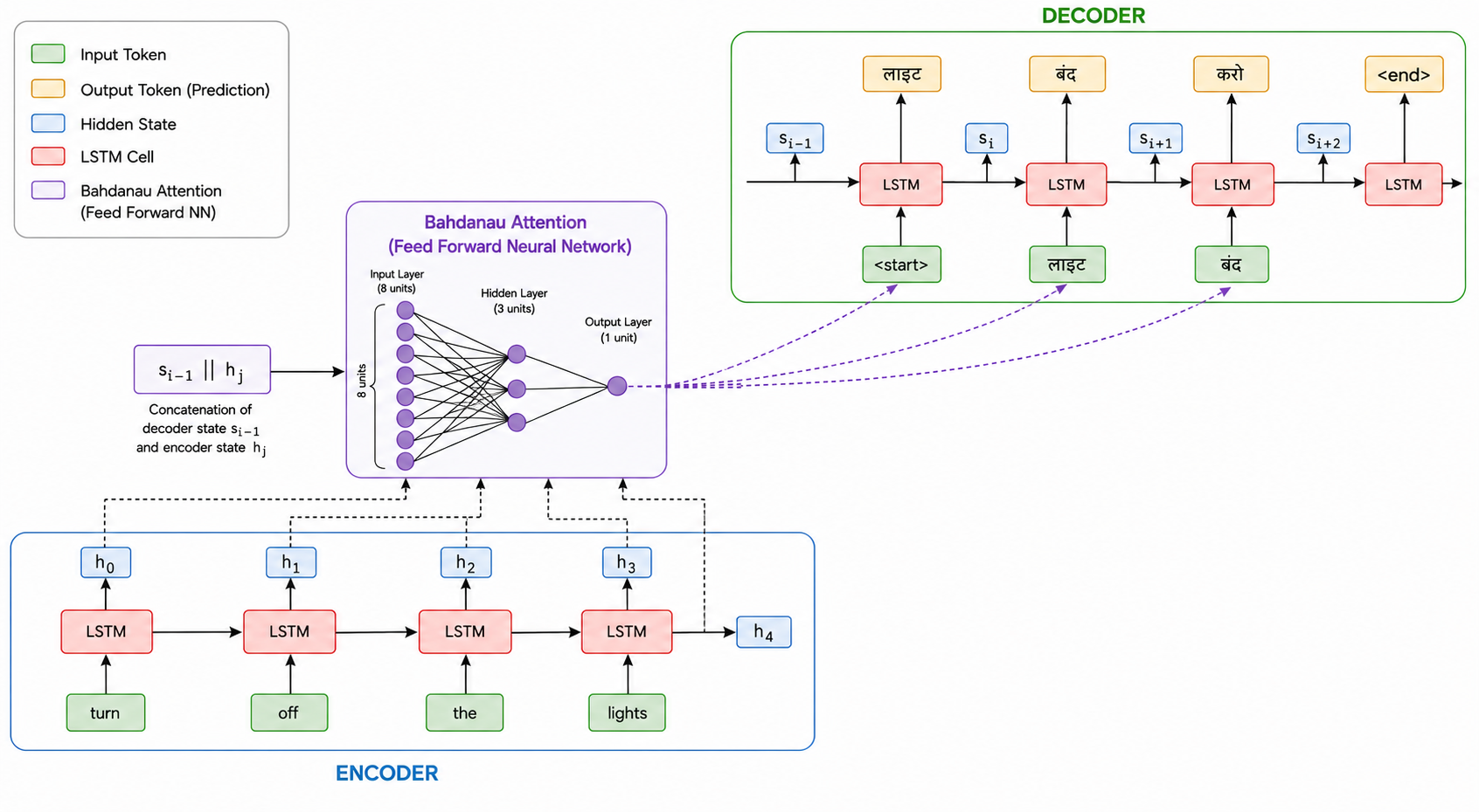
The output of this neural network is a single scalar value:
This is the alignment score. You can think of it as the network's estimate of how relevant the encoder hidden state is for generating the output at decoder step .
Of course, these alignment scores by themselves are not very useful. They can take arbitrary values and cannot yet be interpreted as attention weights. So, just as we discussed in the previous blog, we pass all the alignment scores corresponding to the current decoder step through a softmax layer:
This converts the raw alignment scores into attention weights.
These attention weights are then used to compute the context vector:
And this context vector is what gets supplied to the decoder while generating the output at time step .
Intuitively, tells the decoder how much weight to place on each encoder hidden state while producing the current output. Encoder hidden states with larger attention weights contribute more to , while those with smaller attention weights contribute less.
So, if we zoom out for a second, Bahdanau Attention is essentially a learnable scoring mechanism. Given a decoder state and an encoder state, it learns to assign a relevance score between them. Everything else (the softmax, the attention weights, and the context vector) follows exactly the same pipeline that we already discussed in the previous blog.
A Note on Notation
You'll often see the Bahdanau alignment score written in the literature as:
This looks different from the concatenation-based version we're using, , but the two are mathematically equivalent up to parameterization. Concatenating and and multiplying by a single matrix is the same as multiplying each vector by its own sub-matrix ( and , the two halves of ) and summing the results, since matrix multiplication distributes over concatenation that way. The paper's version simply omits an explicit bias term for notational simplicity; the bias isn't absorbed into , it's just left out, and many practical implementations add one back in regardless. So the difference you see across papers and implementations is purely notational, not architectural.
Computing the Attention Weights for
Now, we can calculate the attention weights needed to construct .
To do this, we compare the previous decoder hidden state with every encoder hidden state , producing a set of alignment scores:
Since we are calculating the context vector for the first decoder step, we need the attention weights:
which means we first need the corresponding alignment scores:
To compute these scores, we feed the decoder hidden state together with every encoder hidden state into the feedforward neural network.
Assume that both and are 4-dimensional vectors. (Real models almost never use vectors this small: hidden-state dimensions in the hundreds or even thousands are typical. We're sticking with 4 purely so the matrices stay easy to read on the page.) For each encoder position , we form the concatenated vector , which is an 8-dimensional vector. When we do this for all four encoder positions simultaneously, we stack these concatenated vectors row-wise into a matrix:
This is a matrix. Each row is the concatenation of with one encoder hidden state, an 8-dimensional vector. We stack four such rows because we have four encoder positions, and each row corresponds to a different encoder position rather than a different training example.
You can think of each row as one comparison between the decoder state and a particular encoder hidden state.
- The first row corresponds to the pair and will be used to calculate .
- The second row corresponds to and will be used to calculate .
- Likewise, the third and fourth rows are used to calculate and respectively.
This entire matrix is fed into the feedforward neural network in one shot. We're processing all four encoder positions simultaneously through matrix operations purely for computational efficiency: there's no batch of training examples here, just one decoder step's worth of comparisons stacked together. Since our network has a single output unit, it produces four alignment scores:
Passing these through a softmax layer gives us the attention weights:
which are then used to compute the context vector .
Inside the Feedforward Neural Network
Here's what actually happens inside this feedforward neural network.
Recall our assumptions:
- The input matrix has shape .
- The hidden layer contains 3 neurons.
- The output layer contains 1 neuron.
Since the input dimension is 8 and the hidden layer contains 3 units, the weight matrix connecting the input layer to the hidden layer will have dimensions:
(Depending on the notation being used, you might sometimes see this written as . The difference is purely a matter of convention. For our discussion, we'll stick with the notation.)
Now, remember that our input matrix is , with each of the four rows corresponding to one encoder position rather than a training example. We process all four rows together through matrix operations purely for computational efficiency; there's no need to loop over them one at a time.
During forward propagation, the first operation is a matrix multiplication:
So after the first layer, we obtain a matrix of shape .
We add the bias terms and apply a non-linearity such as :
Even after this operation, the output still has shape .
Next, this hidden-layer output is multiplied by the weight matrix connecting the hidden layer to the output layer.
Since the hidden layer contains 3 neurons and the output layer contains 1 neuron:
Performing the multiplication gives:
This means that the network produces four scalar outputs:
These are our alignment scores.
Notice that these are not yet attention weights. They are simply raw scores produced by the neural network. They can be positive, negative, large, small, whatever the network decides is appropriate.
To convert them into attention weights, we pass them through a softmax layer:
For our example, this becomes:
and similarly for , , and .
The nice thing about softmax is that:
- Every attention weight becomes positive.
- All attention weights add up to 1.
So after applying softmax, we finally obtain:
These are the attention weights that tell us how much weight to assign each encoder hidden state while generating the first output word.
Once we have these weights, we simply plug them into:
which gives us the context vector .
The attention mechanism has done its job. We now have:
- The context vector ,
- The decoder input token (the start token),
- And the decoder hidden state from the previous step.
At a high level, the decoder update can be written as:
meaning that the previous output token, the previous decoder state, and the context vector jointly determine the next decoder state.
The decoder LSTM then produces:
- The first output word, "लाइट",
- And an updated decoder hidden state .
(As a quick reminder for anyone jumping in without the previous blog: our running example translates the English sentence "Turn off the lights," so the decoder is generating the Hindi words for that sentence one token at a time.)
In other words, not only have we generated the first output token, but we have also updated the decoder's internal state.
Moving to Decoder Time Step 2
Moving forward to the second decoder time step, our goal now is to compute the context vector .
As per the attention equation:
The decoder state has been updated from to since we generated the first output word, "लाइट". So to get the new attention weights , , , and , we concatenate with each encoder hidden state:
Running this matrix through , the bias and activation, and then gives us the alignment scores for this step:
Softmax converts these into the new attention weights, , which we then plug into:
giving us the context vector for decoder time step 2. We now have everything needed by the decoder: , the previous decoder state , and the previously generated output token "लाइट", which is fed back as the decoder input token .
So by the end of decoder time step 2, we have successfully generated the second output word and updated the decoder's internal state once again, and the same cycle continues for the next decoder time step.
The Process Keeps Repeating
Once decoder time step 2 is finished, we move on to decoder time step 3, then 4, then 5, and so on, until the decoder generates the end-of-sequence token.
Here's something worth pausing on: the weights inside the feedforward neural network never change from one decoder time step to another. The same network, the same and , is reused at every decoder step. The weights used to calculate are exactly the same weights used to calculate , and so on for every subsequent step.
So if the weights are staying fixed, why do the attention weights change?
The answer lies in the inputs. The encoder hidden states remain fixed throughout decoding; they were generated once and never recomputed. What keeps changing is the decoder hidden state:
Because the decoder state keeps changing, the input to the feedforward neural network changes at every decoder step. And because the input changes, the alignment scores change, and because the alignment scores change, the attention weights change. That's exactly why the attention distribution can shift from one part of the source sentence to another as the decoder generates different output words.
This also clarifies why the attention weights depend on two things:
The encoder hidden state tells us which part of the source sentence we're looking at, while the decoder hidden state tells us what has already been generated and what the decoder is currently trying to predict. Together, these two pieces of information determine how much attention a particular encoder position receives.
Since the same feedforward network is reused across all decoder time steps with shared parameters, it's often described as a time-distributed fully connected network: the same network applied repeatedly at every decoder step, with the same weights each time.
Of course, these parameters do eventually change, but not during the forward pass. They're only updated after the entire training example has been processed: once the decoder generates the complete output sequence, we compare it against the ground-truth sequence using a loss function such as categorical cross-entropy, and the resulting error is backpropagated through the decoder, the attention mechanism, and the alignment network, updating all the trainable parameters involved. It's worth being precise here: the attention weights themselves are not trainable parameters; they're intermediate values computed fresh on every forward pass. What actually gets updated are the weight matrices ( and ) used to produce the alignment scores that the attention weights are derived from. When the next training example arrives, the same computations happen again, now using the updated weights.
Summarizing the Mathematics
By now, the overall architecture should be fairly clear. Rather than manually repeating the calculations for every remaining decoder time step, we can pause and summarize everything mathematically.
The context vector for decoder step is computed as:
The attention weights are obtained by applying a softmax over the alignment scores:
The only remaining question is: where do these alignment scores come from?
We started by constructing the input matrix: taking the decoder hidden state from the previous time step, , and concatenating it with each encoder hidden state , producing an 8-dimensional vector for each position, then stacking these into a matrix and feeding it into the feedforward neural network.
The first operation inside the network is a multiplication with the input-to-hidden weight matrix . We then add the bias term and apply :
(A quick notational note: throughout the matrix walkthrough above, we treated each row as a row-vector and multiplied on the right by . The equation below is written in the more compact, column-vector form you'll typically see in papers, where multiplies the concatenated vector on the left. The two are just different conventions for writing the same computation; nothing about the underlying math changes.)
where denotes the concatenation of the two vectors. Next, we pass this hidden-layer representation through the output layer with weight matrix , giving the final alignment score:
This single equation captures the entire Bahdanau alignment network.
Putting everything together, the complete Bahdanau Attention mechanism can be summarized as:
Step 1: Compute the alignment scores:
Step 2: Convert them into attention weights:
Step 3: Compute the context vector:
If you understand these three equations, then you understand the complete mathematical formulation of Bahdanau Attention.
A Note on the Alignment Model
The feedforward neural network that we used in Bahdanau Attention has a special name. In the original research paper, it is referred to as the alignment model. Its entire job is to take an encoder hidden state and a decoder hidden state and produce a score that tells us how relevant those two states are to one another.
A Brief Historical Detour
Before attention entered the picture, the earliest encoder-decoder models for sequence-to-sequence tasks compressed the entire input sentence into a single fixed-length vector (the encoder's final hidden state) and asked the decoder to generate the whole output from that one vector alone. This worked reasonably well for short sequences, but it created an information bottleneck: cramming an arbitrarily long sentence into one fixed-size representation meant a lot of detail simply got lost, especially as sentences grew longer.
Bahdanau Attention was introduced specifically to address that bottleneck, letting the decoder look back at all the encoder hidden states instead of relying on a single compressed summary. Luong Attention came shortly after, proposing computational simplifications and alternative scoring functions that kept the same core idea while making it cheaper to compute. Together, these two mechanisms laid much of the conceptual groundwork that later led to self-attention and the Transformer architecture.
The Luong Attention Architecture
Time to discuss the architecture of Luong Attention.
At first glance, it looks very similar to Bahdanau Attention. The encoder remains exactly the same, and even most of the decoder pipeline remains unchanged.
We'll walk through it step by step using our running example.
As usual, the input sentence is fed into the encoder one token at a time:
Turn → off → the → lights
After processing the entire sentence, the encoder produces the hidden states:
With that, the encoder's job is finished.
Now the decoder takes over.
We begin with the initial decoder hidden state . Depending on the implementation, this can either be initialized using the encoder's final hidden state or through some other initialization strategy.
The decoder is first given:
- The start token,
- The previous decoder state .
At a high level, the decoder update can be written as:
Using these inputs, the decoder LSTM computes the current decoder hidden state:
Here's an important difference from Bahdanau Attention. There, we used the previous decoder state to calculate the attention scores. In Luong Attention, we first compute the current decoder state and then use that state to calculate attention. This is exactly the difference we discussed earlier.
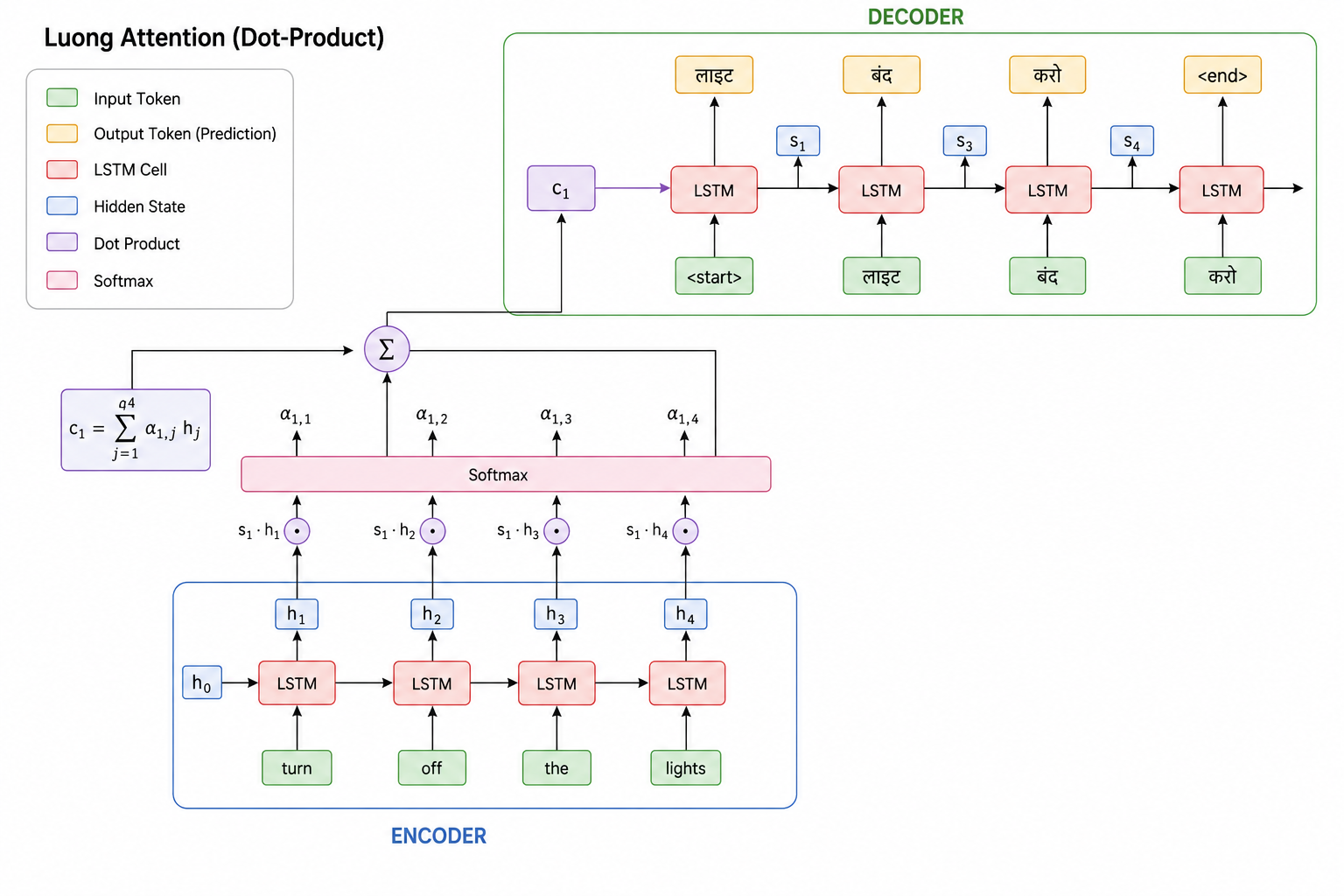
Now we take and compare it against every encoder hidden state using dot products:
This gives us four alignment scores:
These scores are then passed through a softmax layer to obtain the attention weights:
Once the attention weights are available, we compute the context vector:
Up to this point, everything should feel familiar. However, this is where Luong Attention introduces another difference. In Bahdanau Attention, the context vector influences the computation of the next decoder state because attention is computed before the decoder update. Luong Attention takes the opposite approach: it first computes the decoder state and only afterward combines that state with the context vector.
Specifically, we concatenate:
and pass the result through a linear layer followed by a non-linearity. This produces a new vector often called the attentional hidden state, which we'll denote as .
Putting that into an actual equation, this step looks like:
Nothing mysterious going on here, it's exactly the pipeline we just walked through, just written compactly. is the current decoder hidden state, is the context vector we computed from attention, and is the two of them concatenated together, same as before. is just a learnable weight matrix that gets multiplied against this concatenated vector, and the is the non-linearity that squashes the result. Whatever comes out the other side is , the attentional hidden state: the thing that actually goes on to produce the output token, rather than alone.
This attentional hidden state is what is ultimately used to generate the output token. In other words:
rather than directly using alone. The decoder first forms its own opinion about what should be generated next by computing . Then attention is applied, relevant information is gathered from the encoder through , and finally both pieces of information are combined to form the attentional hidden state , which is then used to generate the first output token.
Decoder Time Step 2 in Luong Attention
Once the first output word has been generated, we move on to the second decoder time step. The process is almost identical.
The decoder now takes the previous output token ("लाइट") and the previous decoder state , and computes the next decoder hidden state .
Instead of sending directly to the output layer, we first use it to calculate the attention scores:
These alignment scores are passed through a softmax layer, giving , which we use to calculate the context vector:
Now comes the key architectural step: instead of feeding the context vector into the decoder input, we concatenate it with the current decoder hidden state, , and pass this combined representation through a small feedforward layer to produce the attentional hidden state . This attentional hidden state is used to generate the next output token: "बंद".
At the same time, the decoder state has already been updated to , which will be used to compute the next decoder state . The same process then repeats for the remaining decoder steps until the entire output sequence has been generated.
Why Luong Attention Computes Alignment Scores the Way It Does
Now that we understand Luong Attention, we can talk about the two key differences it introduces.
First Difference: Using the Current Decoder State
In Bahdanau Attention we computed the alignment score using the previous decoder hidden state:
Luong Attention makes a small but meaningful change. Instead of using the previous decoder hidden state, it uses the current decoder hidden state:
The intuition is fairly straightforward: since contains more up-to-date information about the current decoding step, it can potentially make a better decision about which encoder positions deserve attention.
Second Difference: Replacing the Alignment Network
The second difference is even more interesting. In Bahdanau Attention, the function was implemented using the alignment model:
Luong Attention asks a simple question:
Do we really need an entire neural network just to measure how related two hidden states are?
Instead of passing the vectors through an alignment network, the simplest form of Luong Attention directly computes their dot product:
A dot product only works if the two vectors have the same dimensionality, so and need to line up in size. In our running example that's true by construction, but in general the decoder and encoder hidden states won't always match; if they don't, a learned projection matrix can map one of them into the other's space before the dot product is taken.
Suppose:
Then:
which is just a scalar value, and this scalar becomes the alignment score. Once we have all the alignment scores for a decoder step, we apply softmax exactly as before:
and then compute , just like in Bahdanau Attention.
Why Does This Work?
The purpose of the alignment score isn't to perform some complicated transformation, it's simply to measure how relevant an encoder hidden state is for the current decoding step. A dot product already acts as a similarity measure: if two vectors point in similar directions, their dot product tends to be large; if they're dissimilar, it tends to be smaller. Worth noting, though: the dot product depends on both the direction and the magnitude of the two vectors, so it isn't quite the same thing as cosine similarity, which only cares about direction. Even so, it works well in practice as a similarity proxy for measuring how compatible two hidden states are.
So instead of learning a complicated scoring function through a neural network, Luong Attention uses this simpler similarity-based approach. This reduces computation and introduces fewer parameters, making the attention mechanism faster and simpler to train.
Beyond Dot Product: Luong's Other Scoring Functions
It's worth knowing that the original Luong paper didn't propose dot-product attention alone; it introduced a family of scoring functions, with dot product being just the simplest member:
Dot:
General:
Concat:
Dot is the version we just walked through, no learnable parameters, just a raw similarity measure between the two hidden states. General introduces a learnable weight matrix between the two vectors, giving the model some flexibility to learn which dimensions of the hidden states should matter more when computing similarity, while still being far cheaper than a full alignment network. Concat is the closest in spirit to Bahdanau's approach: it concatenates the two hidden states and pushes them through a -activated layer before producing a score, essentially borrowing Bahdanau's alignment model wholesale. In practice, "Luong Attention" is most often used as shorthand for the dot-product variant, since that's the version that captures the efficiency argument the paper is best known for.
The same paper also introduced a separate distinction worth knowing about: global versus local attention. Everything we've covered so far is global attention: at every decoder step, we compute alignment scores against all encoder hidden states. Local attention instead predicts a single position in the source sequence and attends only to a small window of encoder states around it. The motivation is efficiency on long sequences, since scoring every encoder position gets expensive as the input grows. We won't go into the formulas here, but it's worth knowing the dot/general/concat scoring functions and the global/local attention choice are two separate axes of the same paper.
Why Both Mechanisms Exist: A Trade-off, Not a Winner
It's natural to wonder, at this point, why anyone would still reach for Bahdanau Attention once Luong's simpler version exists. The answer is that the two approaches make different bets.
Bahdanau Attention's alignment network is more expressive: a feedforward layer with a non-linearity can learn more complex relationships between decoder and encoder states than a simple dot product can. That expressiveness comes at a cost, though: the alignment model introduces its own weight matrices ( and , or , , and depending on notation) that must be learned, and every alignment score now requires a forward pass through that network rather than a single dot product.
Luong Attention trades some of that expressiveness for simplicity. The dot-product variant needs no additional parameters at all, and computing alignment scores is just a matrix multiplication between the decoder state and the encoder states: cheap, fast, and easy to parallelize. The general and concat variants reintroduce some learnable structure, but even general's single weight matrix is lighter than Bahdanau's full alignment network.
Neither approach is universally better. It comes down to how much capacity your model can afford, how large your dataset is, and how much you're actually gaining from the extra expressiveness on your particular task; gains that, in practice, turned out modest enough that the simpler, cheaper Luong-style mechanisms became the more common default in later work.
Bahdanau vs. Luong: A Side-by-Side Comparison
| Bahdanau Attention | Luong Attention | |
|---|---|---|
| Decoder state used | Previous state, | Current state, |
| Alignment function | Feedforward network with : | Dot, general, or concat (most commonly dot: ) |
| Additional parameters | , (or , , ) | None for dot; for general; , for concat |
| Computational cost | Higher (full forward pass per alignment score) | Lower (dot product is a single matrix multiply) |
| Where context is incorporated | Before computing the decoder state, as an input to it | After computing the decoder state, combined to form |
| Common names | Additive Attention | Multiplicative Attention |
Key Takeaways
- Both Bahdanau and Luong compute attention weights from alignment scores.
- Bahdanau uses a learnable alignment network and the previous decoder state.
- Luong typically uses multiplicative scoring and the current decoder state.
- Both ultimately produce a context vector that helps generate the next output token.
Wrapping Up
And that's Bahdanau Attention and Luong Attention.
At first glance, the differences between the two might seem small. After all, both mechanisms are trying to solve the exact same problem: determining which encoder hidden states are most relevant while generating a particular output token. However, the way they approach that problem is quite different.
Bahdanau Attention uses a learnable alignment model and relies on the previous decoder state to calculate attention scores. Luong Attention simplifies the scoring mechanism, often replacing it with a dot product, and uses the current decoder state instead.
The reason we spent so much time understanding these architectures is that they provide the conceptual bridge to what comes next. When you eventually study self-attention and transformers, many of the ideas will start feeling familiar. The notion of calculating relevance scores, converting them into attention weights, and using those weights to build context-aware representations all originate from the ideas we've discussed in this blog.
Self-attention is at the heart of the Transformer architecture, and having a strong intuition for Bahdanau and Luong Attention makes that journey significantly easier. So if you've understood how the alignment scores are computed, how attention weights emerge from them, and how the context vector influences the decoder, you're in a great position to move forward.
In the next blog, we'll build on these ideas and start exploring attention mechanisms that no longer rely on recurrent networks at all.