Positional Encoding, Explained from First Principles

Self-attention is one of the most brilliant ideas in deep learning.

It lets every token look at every other token, weigh what matters, and build context in a way that feels almost absurdly powerful. In a single mechanism, Transformers got rid of recurrence, made sequence modeling massively parallel, and changed the trajectory of modern machine learning.

But there’s a catch.

A very important one.

And positional encoding exists because of it.

Before we get there, I’ll assume you’re already comfortable with self-attention and multi-head attention, because everything in this blog is built directly on top of them.

If you want a proper refresher, you can check out my previous blog on self-attention here↗.

Now that that's sorted, without any further ado, let's get started.

A small note before we begin

Throughout this blog, whenever I casually say self-attention, I'm essentially referring to the kind of attention mechanism that is actually used in modern Transformers: multi-head self-attention.

So if at some point I say self-attention and at some other point I say multi-head attention, I'm still talking in the context of the Transformer-style attention mechanism we use in practice today.

The problem positional encoding was created to solve

One of the key things self-attention does is allow each token's representation to become context-dependent. Instead of every token carrying a fixed, static embedding, the attention mechanism lets each token look at the other tokens in the sequence and incorporate information from them. That is genuinely powerful.

But it still has a very significant caveat.

Self-attention computes interactions between all token pairs in the sequence in parallel, meaning all of those token-token relationships are computed simultaneously, rather than one step at a time the way RNNs do it. This is one of the biggest reasons Transformers train so efficiently.

But this parallelism comes with a trade-off.

Because self-attention processes all tokens in parallel, it has no built-in notion of order. By itself, it can model how tokens relate to one another, but it has no idea which token came first, which came later, or how far apart two tokens were in the original sequence.

We can make that statement precise by saying that self-attention without positional information is permutation-equivariant. If we write the self-attention block as a function $f$, let $X$ denote the input sequence, and let $\pi$ denote any permutation (that is, any reordering) of the tokens, then:

This equation says that if you shuffle the input tokens before passing them through self-attention, the output representations are shuffled in exactly the same way. In other words, the mechanism treats the input as a set of token vectors rather than an ordered sequence. It can capture interactions between tokens, but it has no native sense of what came before or after anything else.

So a self-attention block, on its own, has no built-in way of distinguishing between:

• the cat chased the dog
• the dog chased the cat

The tokens are exactly the same. The order is completely different. The meaning is entirely different. But without positional information injected from outside, the architecture has no way of knowing that one ordering came before another — the two inputs are structurally indistinguishable to it.

That is the problem.

So we need some way of feeding positional information into the self-attention mechanism.

Let's try to solve it from first principles

To build intuition, let's take a very small example.

Suppose our input is the phrase river bank.

At a high level, a Transformer pipeline first converts each word into an embedding using some embedding mechanism. Word2Vec, a learned embedding table, it doesn't matter for our purposes. So we get:

These are the embedding vectors for the two words. Now we feed them into the self-attention block, which produces new contextualized embeddings for both words, representations that now incorporate information from each other.

Let's assume, purely for illustration, that each embedding is 6-dimensional.

So at this point, the embedding for river is a 6-dimensional vector, and the embedding for bank is also a 6-dimensional vector.

So far, so good.

A very natural first idea

If the problem is that self-attention doesn't know where a word occurred in the sentence, then one very natural idea is:

Why not just attach the position of the word to its embedding?

For example, river occurs at position 1 and bank occurs at position 2. More generally, for a sentence of $n$ words, we assign positions $1, 2, 3, \dots, n$.

So maybe we simply append this positional information to the embedding itself. Since our embedding was originally 6-dimensional, we add one more dimension at the end that stores the word's position:

• the embedding of river becomes a 7-dimensional vector, with the last component storing 1
• the embedding of bank becomes a 7-dimensional vector, with the last component storing 2

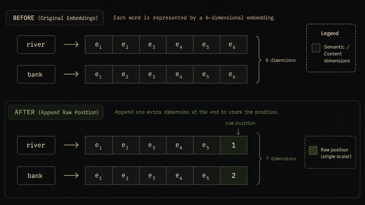
The model now gets both the semantic content of the word and its position. At first glance, this looks pretty reasonable. But it turns out this approach has a few problems.

Problem 1: the raw position value grows with sequence length

Right now our toy example only has two words, so the positional values look harmless. But real sequences can be much longer: 50 tokens, 100, 512 or more. If we store the position as a raw scalar, then later tokens carry values like $48, 49, 50, \dots$ and these numbers keep growing with sequence length.

This is not a great signal to inject into a neural network. A raw, unbounded scalar is a low-capacity, one-dimensional representation of position. It does not scale gracefully to long sequences, and it generalizes poorly when the model is applied to sequence lengths outside the range seen during training.

Using the raw position itself as the positional signal is unbounded and brittle, not the kind of clean, well-behaved input representation we want.

Problem 2: a single scalar is a weak positional signal

Even setting the magnitude issue aside, there is a deeper problem: a single scalar is just not a very rich representation of position.

Think about what the model actually needs to reason about. It needs to know not just "this token is at position 17" but also something about how positions relate to each other: which tokens are nearby, which are far apart, and whether certain positional patterns recur. A single raw integer doesn't capture any of that structure. It's a flat, dimensionless counter, not a distributed representation.

In contrast, the embeddings for words are typically high-dimensional vectors. They live in a rich representational space that captures semantic and syntactic relationships through geometry. Why would we settle for a single scalar to represent something as important as position?

What we really want is a positional representation that is distributed, multi-scale, and structured, not a single raw number.

Problem 3: it does not naturally capture relative position

This is the final problem, and it is the most important one.

There are two kinds of positional information we might care about.

Absolute position means the exact position of a word in the sentence. For example, in I see the sun, the word I is at position 1, see is at position 2, and so on.

Relative position means the position of one word with respect to another, that is, the distance between words. If two words are adjacent, that is one kind of relationship. If they are 5 tokens apart, that is another.

Relative position matters a lot in language. Nearby words often have strong syntactic and semantic dependencies. What we would really like is a positional representation that makes it easy for the model to reason about how far apart two tokens are, and whether certain structural patterns repeat at fixed offsets.

A raw scalar like 1, 2, 3, 4, ... does not expose any of that structure in a clean way.

So by now, our naive solution has run into three real issues.

So what kind of positional function do we actually want?

Based on the problems above, we can start designing something better.

Ideally, we want a function that is:

1. Bounded — values stay within a fixed range regardless of sequence length.
2. Rich and multi-scale — not a single scalar, but a distributed representation that captures positional information at multiple granularities.
3. Structured with respect to relative offsets — so that the encoding at position $\text{pos} + k$ has a predictable relationship to the encoding at position $\text{pos}$, for any offset $k$.

So the question becomes: is there a class of functions that gives us all three of these things?

Yes. And the answer comes from one of the most familiar corners of mathematics.

Trigonometric functions to the rescue

Functions like sine and cosine are exactly the kind of objects we're looking for.

They are bounded: $-1 \leq \sin(x) \leq 1$ always, regardless of how large $x$ gets. They are smooth and continuous: no abrupt jumps. And they are periodic: $\sin(x + 2\pi) = \sin(x)$, meaning the pattern repeats at a fixed interval.

These properties already make sinusoids a much better candidate than a raw scalar. But there is something deeper going on too. Sinusoids have a beautiful mathematical relationship between values at different positions that makes them especially well-suited for encoding relative structure. We will get to that properly once the full formula is in place. For now, the key thing to notice is that sine and cosine give us a bounded, smooth, structured signal, exactly what we were asking for.

The next natural idea: pass position through a sine function

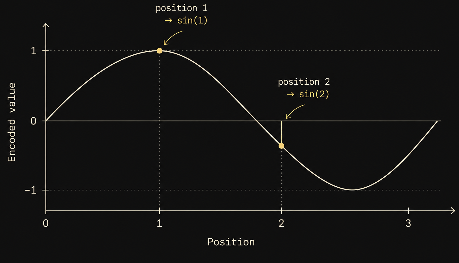
With that motivation in place, suppose we take the position of each word and pass it through a sine function. So instead of storing the raw position, we store $\sin(\text{pos})$.

For our toy example:

• river is at position 1 → $\sin(1)$
• bank is at position 2 → $\sin(2)$

The values are now bounded between $-1$ and $1$, continuous, and periodic. This already feels like a much better positional signal than raw integers.

But we've introduced a new problem.

The problem with a single sine value

Since sine is periodic, its values repeat: $\sin(x) = \sin(x + 2\pi k)$ for integer $k$. So if we represent position using only one sine value per token, different positions can end up with the same encoded value once the sequence gets long enough. The encoding is no longer reliably distinct.

And a single scalar, even a sine of the position, still gives us essentially one number per token. That's a very low-dimensional positional signal.

We need something richer.

First improvement: use both sine and cosine

A natural fix is to use both:

Using both sine and cosine is better than using sine alone because together they capture the phase of the oscillation more completely. But a single frequency still repeats too quickly to serve as a robust positional representation for long sequences, which is why the Transformer uses many frequencies at once.

But we can push this further.

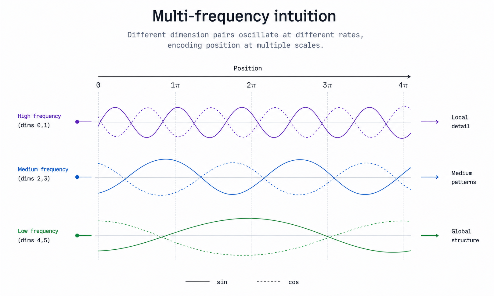
Second improvement: use multiple frequencies

Why stop at one frequency? For a position $p$, we could compute:

Now we're representing each position as a vector of sinusoidal values at different frequencies. Instead of "position 7 is the number 7" or "position 7 is $\sin(7)$", we're saying:

Position 7 is a whole pattern of sine and cosine values — one per frequency — and that pattern is essentially unique to position 7.

That is much richer and much harder to confuse with any other position.

But this creates a dimensionality problem

If we keep concatenating more sine/cosine values onto the token embedding, the embedding dimension keeps growing. That is not what we want. The downstream architecture expects a fixed embedding size.

So the real question is:

Can we construct a positional vector using sine and cosine values at different frequencies without inflating the embedding dimension?

Yes. And this is where the actual Transformer solution comes in.

A critical conceptual point: positional encoding is tied to position, not to the word

Before we get to the formula, there is one distinction worth making explicit.

Positional encoding is not a property of the word. It is a property of the position in the sequence.

That means if the same word appears twice in a sentence, both occurrences use the same token embedding, but they get different positional encodings because they are at different positions.

For example, in the dog chased the ball, the word the appears at positions 0 and 3. Both occurrences share the same token embedding $E(\text{the})$, but they receive different positional encodings:

• first the → $E(\text{the}) + PE(0)$
• second the → $E(\text{the}) + PE(3)$

This is how the model distinguishes the two.

Positional encodings don't need to be globally unique

They only need to be distinguishable within the sequence lengths the model is expected to handle. Two tokens in two completely different sentences can share the same positional encoding. What matters is that positions within any single sequence are distinct.

The actual Transformer solution: addition, not concatenation

Here is the key design choice.

Suppose the token embedding dimension is $d_{\text{model}} = 512$. Every token embedding is a vector in $\mathbb{R}^{512}$. The Transformer constructs a positional encoding vector of the same dimension, also in $\mathbb{R}^{512}$, and then adds the two elementwise:

This one operation is the whole idea.

• $E(\text{token}_i)$ encodes **what the token is**
• $PE(i)$ encodes **where it is in the sequence**
• $x_i$ carries both, and is still a $d_{\text{model}}$-dimensional vector

Contrast this with concatenation, which would produce a vector of dimension $d_{\text{model}} + d_{\text{PE}}$. If both are 512-dimensional, concatenation gives you a 1024-dimensional vector. Addition keeps the dimension fixed at 512.

The Transformer uses addition. The embedding dimension does not change.

So what does $d_{\text{model}}$ actually mean?

When we say "$d_{\text{model}} = 512$" or "512-dimensional embedding", we simply mean the vector contains 512 components:

The token embedding, the positional encoding, and their sum are all 512-dimensional. Nothing inflates.

We've reached the actual solution

All of that groundwork was worth it. We now have exactly the background we need to understand the formula from the Attention Is All You Need paper.

The actual setup

Our sentence is river bank. Before sending the embeddings into the self-attention block, we want to inject positional information:

Since every token embedding in our toy example is 6-dimensional, the positional encoding vectors must also be 6-dimensional. So the question is simply:

How do we construct a 6-dimensional positional encoding vector for each position?

Filling the positional encoding vector in pairs

If the positional encoding vector has 6 dimensions, we fill those 6 dimensions in pairs:

• dimensions 0 and 1 → one sine-cosine pair
• dimensions 2 and 3 → another sine-cosine pair (different frequency)
• dimensions 4 and 5 → yet another sine-cosine pair (yet another frequency)

For each pair: the sine value goes into the even-indexed dimension, the cosine value goes into the odd-indexed dimension. And both are evaluated at the token's position.

That is the core idea. Every pair of dimensions contributes one "frequency channel" of positional information.

The formula

If you open the original Attention Is All You Need paper and go to the Positional Encoding section, you find:

At first glance this can look a little intimidating. But after all the discussion above, it is saying exactly the same thing we just described:

• fill alternate dimensions using sine and cosine
• use the token position as the input
• change the frequency as you move from one dimension pair to the next

Let's decode every symbol.

Breaking the formula down, one symbol at a time

What does $\text{pos}$ mean?

• river → $\text{pos} = 0$
• bank → $\text{pos} = 1$

What does $d_{\text{model}}$ mean?

What does $i$ mean?

• $i = 0$ → filling dimensions 0 and 1
• $i = 1$ → filling dimensions 2 and 3
• $i = 2$ → filling dimensions 4 and 5

More generally, $i$ runs from $0$ to $\frac{d_{\text{model}}}{2} - 1$.

Why $2i$ and $2i+1$?

Because the vector is filled two dimensions at a time, one sine slot and one cosine slot:

• $PE(\text{pos},\; 2i)$ → the sine dimension of pair $i$
• $PE(\text{pos},\; 2i+1)$ → the cosine dimension of pair $i$

When $i = 0$: fills dimensions 0 and 1. When $i = 1$: fills dimensions 2 and 3. And so on.

What is the denominator doing?

This controls the frequency of the sine and cosine curves used for each dimension pair.

When the denominator is small, the argument of sine changes quickly as $\text{pos}$ increases, which is a high-frequency wave. When the denominator is large, the argument changes slowly, which is a low-frequency wave.

As $i$ increases, the exponent $2i/d_{\text{model}}$ increases, making the denominator larger, and the corresponding wave lower in frequency. So:

• early dimension pairs → higher frequency (waves oscillate quickly)
• later dimension pairs → lower frequency (waves oscillate slowly)

This gives the positional encoding a multi-scale structure: some dimensions are sensitive to small local shifts in position, while others change gradually and capture broader positional patterns.

Why specifically 10000?

It is a design choice from the original paper. The value 10000 creates a large enough spread of frequencies that the resulting wavelengths range from very short (sensitive to individual token shifts) to extremely long (barely changing across the full sequence). The exact value is not sacred — the point is to span a wide enough range of scales to be useful. The original authors found that 10000 works well in practice.

Why sinusoidal encodings are elegant for relative positions

Earlier, I mentioned that one of the key properties we wanted was that the encoding at position $\text{pos} + k$ should have a predictable relationship to the encoding at position $\text{pos}$. This is where the sinusoidal formula really earns its keep.

For a single frequency $\omega = 1/10000^{2i/d_{\text{model}}}$, the angle addition formulas tell us:

In plain English: if you know $PE(\text{pos})$, you can compute $PE(\text{pos} + k)$ by a linear transformation whose coefficients depend only on $k$, not on $\text{pos}$. The transformation that takes you from "position $\text{pos}$" to "position $\text{pos} + k$" is the same regardless of where in the sequence you are.

This is a very clean mathematical property. It means the model has, baked into the structure of these encodings, a way to reason about relative offsets between tokens. It is not magic — attention layers still have to learn to exploit this structure — but sinusoidal encodings give the model a good starting point.

This is one of the elegant mathematical properties of sinusoidal encodings, and one of the reasons they are such a clean positional scheme to study and understand.

Now let's actually apply the formula

Our sentence is river bank, with $d_{\text{model}} = 6$ and 0-based indexing.

• river → $\text{pos} = 0$
• bank → $\text{pos} = 1$

Since $d_{\text{model}} = 6$, the index $i$ takes the values $0, 1, 2$.

Step-by-step: positional encoding for river ($\text{pos} = 0$)

$i = 0$:

$i = 1$:

$i = 2$:

So:

This alternating pattern makes sense: when $\text{pos} = 0$, the numerator is always 0, so every sine term evaluates to $\sin(0) = 0$ and every cosine term evaluates to $\cos(0) = 1$, regardless of the denominator.

Step-by-step: positional encoding for bank ($\text{pos} = 1$)

Now the numerator is 1, so the different denominators actually produce different values. This is where the multi-frequency structure kicks in.

$i = 0$:

$i = 1$: Since $\frac{2}{6} = \frac{1}{3}$ and $10000^{1/3} \approx 21.54$, the argument is $\frac{1}{21.54} \approx 0.04642$.

$i = 2$: Since $\frac{4}{6} = \frac{2}{3}$ and $10000^{2/3} \approx 464.16$, the argument is $\frac{1}{464.16} \approx 0.002154$.

So:

Notice the pattern: the early dimensions (high frequency) change a lot between $\text{pos} = 0$ and $\text{pos} = 1$, while the later dimensions (low frequency) change very little. This is the multi-scale structure in action — the encoding looks at position from multiple "zoom levels" simultaneously.

Final takeaway

So if I had to summarize the entire idea of positional encoding in one simple flow:

• self-attention is powerful, but without positional information it is permutation-equivariant: it cannot distinguish different orderings of the same tokens
• so we inject positional information by constructing a positional encoding vector for each token position
• instead of using a raw scalar, the Transformer represents each position as a sinusoidal vector, a vector of sine and cosine values at different frequencies
• that vector has the same dimensionality as the token embedding, so we can simply add the two together without changing the dimension
• the frequencies decrease as you move to later dimension pairs, giving the encoding a multi-scale structure
• sinusoidal encodings have a beautiful relative-offset property: the encoding at position $\text{pos} + k$ can be expressed as a linear transformation of the encoding at $\text{pos}$, with coefficients depending only on $k$

So positional encoding is essentially the Transformer's way of telling the model:

"I'm not just giving you the meaning of this token — I'm also telling you where this token occurred in the sequence."

A note on modern positional encoding

One more thing worth saying clearly: what we've walked through here is the sinusoidal positional encoding from the original Attention Is All You Need paper. It is the foundational scheme, and understanding it deeply is the right place to start.

But modern Transformer variants often use different positional encoding strategies. Some of the most common alternatives include:

• Learned positional embeddings — instead of a fixed formula, the model learns the positional encodings from data (used in BERT and several other early Transformer variants)
• Relative positional encodings — encode position differences rather than absolute positions
• RoPE (Rotary Position Embedding) — rotates the query and key vectors by an angle determined by position, achieving the relative-offset property in a particularly elegant way; widely used in modern LLMs
• ALiBi (Attention with Linear Biases) — adds a position-dependent bias directly to the attention scores rather than modifying the embeddings

Each of these is a different answer to the same core question: how do we give the model a useful sense of where tokens are? Sinusoidal encoding is the original, principled answer. The others are refinements and alternatives that have emerged as practitioners have pushed the frontier further.

At first glance, the formula can definitely look scary. But if you build it step by step — first understanding the problem, then understanding why we need sine and cosine, then understanding the multi-scale and relative-offset properties, and finally plugging values into the actual formula — positional encoding starts feeling much more intuitive than mysterious.

And that's exactly the point where I wanted us to arrive.